Linear Regression — Fitting a Line, and Training It
A regression predicts a number — one drawn from infinitely many possible outputs —
rather than a yes/no label. Linear regression does it with the simplest object that can
carry a trend: a straight line. This note builds it from the ground up: the model and its
two parameters, the cost that scores a candidate line, gradient descent and the derivatives
that drive it, the jump to many input features (where vectors, the data matrix and NumPy
earn their keep), the two preparation steps that decide whether training actually works —
feature scaling and feature engineering — and finally regularization, which keeps the
weights from growing wild.
In one line. Linear regression fits $f_{w,b}(x) = wx + b$ by choosing the $w$ and $b$ that minimise the squared-error cost $J(w,b) = \frac{1}{2m}\sum_i (f_{w,b}(x^{(i)}) - y^{(i)})^2$, walking downhill with gradient descent; with $n$ features the line becomes a plane, $f_{\vec{w},b}(\vec{x}) = \vec{w}\cdot\vec{x} + b$, and nothing else changes.
- What a regression predicts
- Defining the model
- The cost function
- Optimising the cost
- Gradient descent for linear regression
- Running gradient descent well
- Multiple feature linear regression
- Vectorization
- The data matrix: the whole training set at once
- Gradient descent for multiple linear regression
- The normal equation: an alternative to gradient descent
- Feature scaling
- Feature engineering
- Regularized linear regression
- Where this goes next
What a regression predicts
Some of the most common algorithms in machine learning are regressions. A regression predicts a number from infinitely many possible number outputs — a price, a temperature, a duration — as opposed to a classification, which picks from a small set of labels.
A linear regression fits a straight line to a dataset; a non-linear regression fits a curved one. When the model uses a single input variable it is called univariate linear regression, though models can, and usually do, have many more than one. The running example here is the practical one: predicting home prices from their square footage.
The data are $m$ training examples, each a pair $(x^{(i)}, y^{(i)})$ — an input (size) and the true output (price). Fitting means finding the line that passes as close to those points as it can.
Defining the model
The line and its two parameters
The function defining a linear regression model is a line:
Here $w$ is the slope — how many thousands of dollars a home gains per extra thousand square feet — and $b$ is the y-intercept, the value the line takes at $x = 0$. These two numbers are the parameters of the model: they are all the algorithm gets to choose, and together they pin the line's direction and position.
The predicted output
Once the line is fitted, the same function definition is applied to make predictions. The only thing that changes is the name of the output: it is no longer an observed truth but an estimate read off the regression line, written $\hat{y}$ ("y-hat") to keep it distinct from the actual $y$:
Keeping $\hat{y}$ and $y$ separate is the whole game. $y^{(i)}$ is what the house sold for; $\hat{y}^{(i)}$ is what the line says it should have sold for. Training is the business of squeezing the gap between them.
Notation
| Symbol | Meaning |
|---|---|
| $x$, $y$ | input feature, output target |
| $x^{(i)}$, $y^{(i)}$ | the input and output of the $i$-th training example |
| $m$ | number of training examples |
| $\hat{y}^{(i)}$ | the prediction for example $i$; also written $f_{w,b}(x^{(i)})$ |
| $w$, $b$ | the parameters: slope (weight) and y-intercept (bias) |
| $J(w,b)$ | the cost — how badly the line $(w,b)$ fits the data |
| $\alpha$ | the learning rate — the size of a gradient-descent step |
| $n$ | number of features, once there is more than one |
| $\vec{w}$, $\vec{x}$ | the weight and feature vectors, each of length $n$ |
| $x_j^{(i)}$ | the value of feature $j$ in the $i$-th training example |
| $\lambda$ | the regularization parameter |
The cost function
The error of one prediction
Since the slope $w$ and the y-intercept $b$ dramatically influence the position and direction of the line, making sure it fits the data as accurately as possible is the central task. Measuring how well a line fits is the job of the cost function.
The error itself lives in the difference between the predicted output and the actual one:
This is a signed number: positive when the line sits above the data point, negative when it sits below.
Squaring and averaging
A single error is not enough — the line must be scored against every example, from $i = 1$ up to the number of training examples $m$. Errors are squared before they are added up, for two reasons: squaring makes every contribution positive (so an overshoot cannot cancel an undershoot into a false zero), and it punishes a large miss far more than a small one.
As the number of examples grows, the total keeps growing with it — a thousand well-fitted points would score worse than ten badly-fitted ones. So the sum is turned into an average, which makes the score comparable across datasets of different sizes. The result is the squared error cost function $J$:
Why divide by $2m$
Dividing by $m$ gives the mean. The extra factor of $2$ is a convenience: it exists purely so that the derivative comes out clean. Differentiating a square brings a factor of $2$ down in front, and that $2$ cancels the $2$ in the denominator — see §5.2. The cost most engineers use therefore divides by $2m$, because it makes the calculations neater further into the process.
Withholding the extra two is perfectly acceptable. Halving a cost does not move its minimum: if $J$ is smallest at some $(w,b)$, so is $\tfrac{1}{2}J$. The $2$ changes the value of the cost and the scale of its gradients, never the location of the best line — which is the only thing being solved for.
While different applications use different types of cost, squared error is easily the most common choice for regression problems.
The cost in terms of the parameters
To see the parameters that are actually being adjusted, substitute the model back in for $\hat{y}^{(i)}$:
The only difference is that the predicted output $\hat{y}$ is now written as the function model $f_{w,b}(x^{(i)})$. Because the model contains the only quantities that can be adjusted — the slope and the y-intercept — this is the complete definition of the cost. The data $x^{(i)}$ and $y^{(i)}$ are fixed; $J$ is a function of $w$ and $b$ alone.
Three candidate lines on the seven homes of Figure 1 make the point concrete:
| Line | $w$ | $b$ | $J(w,b)$ |
|---|---|---|---|
| too flat | $100$ | $100$ | $2028.6$ |
| too steep, through the origin | $160$ | $0$ | $435.7$ |
| the fitted line | $132.1$ | $73.9$ | $\mathbf{38.5}$ |
Optimising the cost
The objective
The goal of a linear regression algorithm is to minimise the cost function — to make it as small as possible by choosing the two parameters that affect it:
Everything from here on is machinery for solving that one line.
The bowl: surface and contours
$J$ can be plotted against each parameter individually, which gives a 2D graph for each — and in both cases a parabola, because the cost is quadratic in its parameters. Holding $b$ at its best value and sweeping $w$ traces one bowl-shaped curve; holding $w$ and sweeping $b$ traces another.
Each curve bottoms out at the fitted value (the green dot), where the cost is $J = 38.5$ — they are two slices through the same bowl.
To get the full picture, however, the two parameters are plotted together, which needs either a 3D surface graph or its 2D shadow, a contour graph. The surface is a bowl; the contours are the level curves you would see looking straight down into it, each ellipse a set of $(w, b)$ pairs that cost exactly the same.
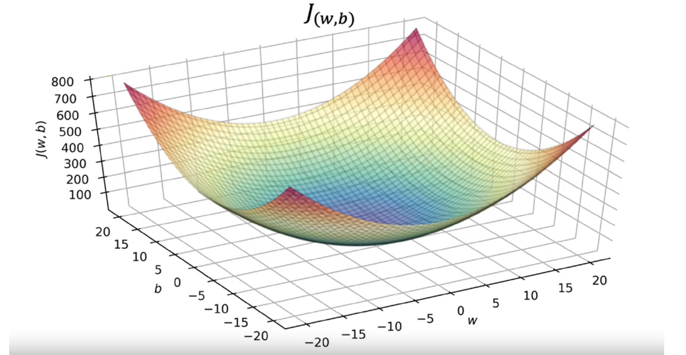
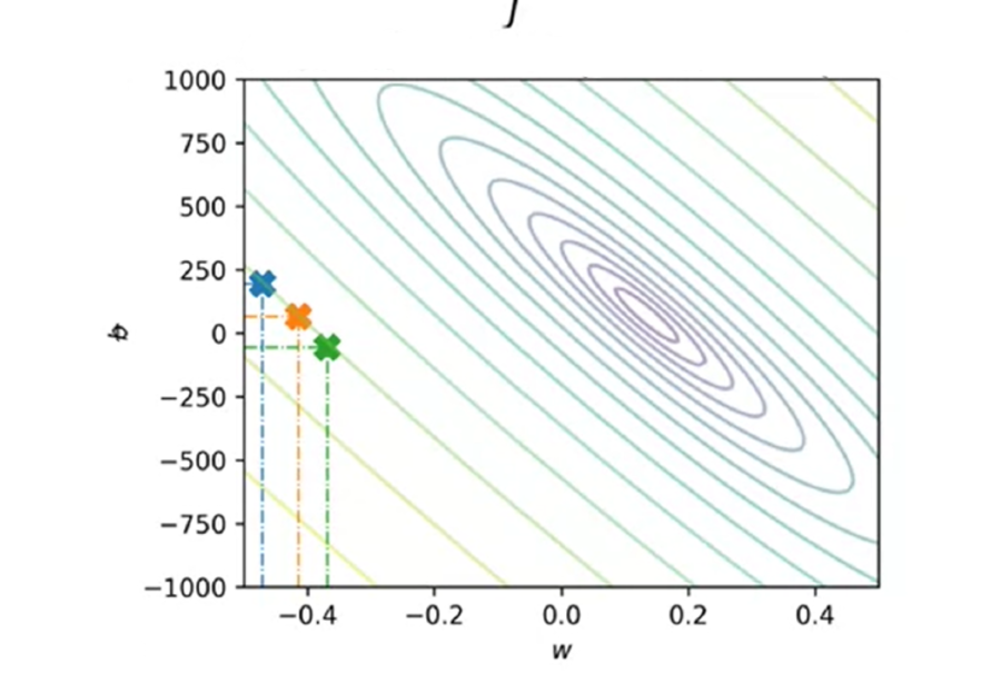
Both pictures show the same object, and minimising $J$ is the same act in either: walking in from the outer, expensive rings until you reach the middle. Because the squared-error cost of a linear model is convex — a single bowl with no local dips to get stuck in — gradient descent started anywhere will roll to the one global minimum.
Gradient descent for linear regression
Given all the definitions above, almost everything is present to compute a linear regression programmatically. One piece is missing: expressions for the derivatives of the cost, $\frac{\partial}{\partial w}J(w,b)$ and $\frac{\partial}{\partial b}J(w,b)$.
The update rule
Gradient descent repeatedly nudges each parameter against its slope — downhill:
The learning rate $\alpha$ sets the step size. The minus sign is what makes it descent: where the cost rises with $w$, the slope is positive and $w$ is pushed down; where the cost falls with $w$, the slope is negative and $w$ is pushed up.
The two derivatives
Since the cost and the model are already expressed in terms of the inputs $x$ and $y$, they can be substituted into the update and the derivative taken directly.
Where the derivatives come from. Start from the cost with the model substituted in, $J(w,b) = \frac{1}{2m}\sum_{i=1}^{m}\left(w\,x^{(i)} + b - y^{(i)}\right)^{2}$, and differentiate one term of the sum by the chain rule. The outer function is a square, whose derivative brings down a factor of $2$; the inner function is $w\,x^{(i)} + b - y^{(i)}$, whose derivative with respect to $w$ is $x^{(i)}$ and with respect to $b$ is $1$. The factor of $2$ that comes down from the square cancels the $2$ in the $2m$ — which is exactly why that $2$ was put there in the first place.
Both gradients are averages of the error. The only difference is that the $w$-gradient weights each error by its input $x^{(i)}$ — which is exactly right: an example with a large input feels a big change when the slope moves, so it deserves a big say in where the slope goes. The bias sees every example equally, because moving $b$ shifts the whole line by the same amount no matter where the point sits.
The final algorithm
Substituting those two results into the update rule gives the algorithm in the form you can actually code:
Repeat until convergence. One subtlety matters more than it looks: the two updates must be simultaneous. Both gradients are computed from the old $(w, b)$, and only then are both parameters overwritten. Updating $w$ first and letting the new $w$ leak into the gradient for $b$ is a different — and wrong — algorithm.
for _ in range(iterations):
    err   = [w * x + b - y for x, y in zip(X, Y)]   # f(x) - y, one per example
    dw    = sum(e * x for e, x in zip(err, X)) / m  # dJ/dw
    db    = sum(err) / m                            # dJ/db
    w, b  = w - alpha * dw, b - alpha * db          # simultaneous update
The computation graph
The same algorithm read as a graph: the forward pass pushes one example through the model to a cost, and the backward pass walks the same edges in reverse, multiplying local slopes to collect $\partial J/\partial w$ and $\partial J/\partial b$.
A run of the algorithm
Run the update on the seven homes of Figure 1, starting from $w = 0$, $b = 0$ with $\alpha = 0.1$. The cost collapses in the first few iterations and then crawls: the slope $w$ is nearly right after two steps, while the intercept $b$ takes thousands more to drift up to its final value, because the $b$-direction of the bowl is far shallower than the $w$-direction.
| Iteration | $w$ | $b$ | $J(w,b)$ |
|---|---|---|---|
| $0$ | $0.000$ | $0.000$ | $90492.86$ |
| $1$ | $114.286$ | $40.429$ | $3251.11$ |
| $2$ | $135.607$ | $48.243$ | $189.45$ |
| $3$ | $139.517$ | $49.945$ | $81.10$ |
| $5$ | $140.206$ | $50.837$ | $75.33$ |
| $8$ | $139.944$ | $51.690$ | $72.69$ |
| $2000$ | $132.143$ | $73.929$ | $\mathbf{38.52}$ |
Watching a single parameter descend shows the same shape from the side — the steps are large where the bowl is steep and shrink as the slope flattens toward the minimum, even though $\alpha$ never changes:
Running gradient descent well
Everything in §5 was specific to linear regression — the derivatives came from this cost. The algorithm itself is far more general, and so are the things that can go wrong with it. This section is about the algorithm as a tool: what it minimises, how to choose $\alpha$, and how to tell from the outside whether a run is working.
It minimises any function
Gradient descent is used across the whole of machine learning, from fitting a line to training the largest neural networks. Nothing in the update rule mentions a line, a squared error, or even a dataset. Its goal is simply:
Linear regression is the friendly case: its cost is a convex bowl, so there is exactly one minimum and every starting point rolls into it. In general there is no such promise. As the number of parameters grows the surface develops ridges, plateaus and several separate valleys, and the algorithm can only ever walk downhill from wherever it happens to start.
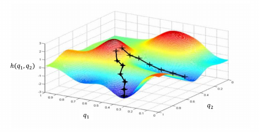
A local minimum is the bottom of one valley; the global minimum is the lowest point on the whole surface. Standard practice is to run the algorithm several times from different random starting points and keep the best result. For the cost in this note the distinction is academic — a squared-error cost on a linear model has a single bowl, which is one of the reasons linear regression is such a good place to learn the algorithm.
The learning rate
$\alpha$ controls how far each step travels, and it is usually a small positive number between $0$ and $1$. It is also the single parameter most likely to ruin a run, in two opposite ways.
- Too small and the algorithm still works — it just takes far more iterations than it needs to, and the total training time grows dramatically.
- Too large and a step overshoots the minimum and lands somewhere with a higher cost. The next gradient is then larger still, so the following step is bigger, and the run diverges instead of converging.
The usual search is a coarse ladder: try $0.001$, then $0.01$, then $0.1$, then $1$, watching the cost after a handful of iterations, and settle just below the value that starts to misbehave.
Why a fixed $\alpha$ is enough. It looks as though the step size ought to shrink as you approach the minimum — otherwise the last step would jump straight past it. It does shrink, automatically, and nothing has to be adjusted. The step length is $\alpha$ times the derivative, and the derivative is the slope of the tangent line at the current $w$. Near the bottom of the bowl that tangent flattens out, so the slope tends to $0$ and each successive step is shorter than the last. Gradient descent glides to a stop on its own; at an exact minimum the derivative is $0$, there is nothing left to subtract, and the parameters stop moving. That is what "convergence" means here.
The learning curve
The most useful diagnostic costs one line of code: record $J$ after every iteration and plot it against the iteration number. That plot is the learning curve, and it says at a glance whether the run is healthy.
The rule for reading it is short: $J$ must decrease on every single iteration. If the curve ever rises, something is wrong — nearly always an $\alpha$ that is too large, occasionally a bug. If it falls and then flattens, the run has converged and further iterations are wasted effort.
How many iterations that takes varies enormously between problems — thirty for the example above, hundreds of thousands for a large model — which is why the number is found by looking at the curve rather than guessed in advance.
The automatic convergence test
The same judgement can be automated. Pick a small threshold $\epsilon$, and stop as soon as one iteration fails to buy enough progress:
The catch is choosing $\epsilon$: too large and it stops early, on parameters that were still improving; too small and it never triggers. In practice the test is used alongside the learning curve rather than instead of it — the curve tells you what a reasonable $\epsilon$ looks like for this problem.
Debugging a run
A cost that climbs or oscillates is usually a learning rate that is too large, but it can just as easily be a bug — a sign error in a gradient, or a non-simultaneous update (§5.3). There is a clean way to tell the two apart:
Set $\alpha$ absurdly small and run again. With a tiny enough step, a correct implementation is guaranteed to decrease $J$ on every iteration — slowly, but monotonically, because a small enough step downhill always goes downhill. If the cost still rises or wanders with a minuscule $\alpha$, the learning rate was never the problem: the gradient itself is wrong. This is a diagnostic, not a fix — once it has told you which of the two you are dealing with, put $\alpha$ back.
Multiple feature linear regression
Adding more input features is a critical component of achieving accurate models. Take the home-price example: square footage alone provides real insight, but it is probably not enough for practical use. Number of bedrooms, number of bathrooms, age, location — each carries information the size cannot.
Notation for many features
Slight modifications to the notation are necessary once there is more than one input:
| Symbol | Meaning |
|---|---|
| $x_j$ | the $j$-th feature |
| $n$ | the number of features |
| $\vec{x}^{(i)}$ | the features of the $i$-th training example — a vector of length $n$ |
| $x_j^{(i)}$ | the value of feature $j$ in the $i$-th training example — a scalar |
The model
With multiple variables comes a necessary update to the model function. Every feature gets its own weight, and the products are summed:
Each $w_j$ now reads as the price impact of one unit of feature $j$, holding the others fixed: dollars per square foot, dollars per bedroom, and so on. The bias $b$ is still a single number — the baseline the features are added to.
Vector form: the dot product
To simplify the notation, collect the parameters and the features into vectors:
Notice that $b$ is not part of $\vec{w}$: it is just a number, not one of the $n$ weights that pair off against features. It is, however, part of the complete model, which now reads as a dot product plus that number:
The dot product is precisely "multiply the matching entries and add them all up" — the same arithmetic as before, written in one symbol instead of $n$ terms. The single-variable model is the special case $n = 1$.
Vectorization
Writing vectorized code is essential for turning these linear-algebra equations into something a computer can run quickly. It also happens that GPUs are extremely efficient at exactly this kind of code.
Three ways to write the same model
Take $n = 3$, with $\vec{w} = \begin{bmatrix} 1.0 & 2.5 & -3.3 \end{bmatrix}$, $b = 4$ and $\vec{x} = \begin{bmatrix} 10 & 20 & 30 \end{bmatrix}$. In code the parameters and features become arrays:
w = np.array([1.0, 2.5, -3.3])   # the n weights
b = 4                            # the bias is a plain number
x = np.array([10, 20, 30])       # the n features of one example
Without vectorization, the sum $\left(\sum_{j=1}^{n} w_j x_j\right) + b$ is spelled out as a loop, one product at a time:
f = 0
for j in range(n):      # 0 to n-1
    f += w[j] * x[j]
f += b
With vectorization, the same dot product is a single call:
f = np.dot(w, x) + bWatch the index base. The linear algebra counts features from $1$ ($w_1 \ldots w_n$) while Python counts from $0$ (
w[0] … w[n-1]). The formula's $w_j x_j$ is the code'sw[j-1] * x[j-1]— one of the quietest sources of off-by-one bugs when transcribing a derivation into an implementation.
NumPy is what makes the vectorized line possible; without it, the multiplication between
$\vec{w}$ and $\vec{x}$ would have to be hard-coded, which becomes especially painful for a
large $n$.
Why vectorized code is faster
The benefit is not only cleaner and simpler code — the performance is genuinely better,
because NumPy uses the parallel hardware in the computer.
Consider the loop above. It runs linearly: it adds the product of $w$ and $x$ for
feature $j$, then for $j+1$, step after step, f += w[j] * x[j] one at a time. With
vectorization, the products for all $j$ are computed in parallel, and specialised
hardware then adds them together to give the final $f$. The gap widens with $n$, and it is
the reason a model with thousands of features is still trainable.
| Form | Mathematics | Python |
|---|---|---|
| Written out | $w_1x_1 + \cdots + w_nx_n + b$ | f = w[0]*x[0] + ... + b |
| Sum, no vectorization | $\left(\sum_{j=1}^{n} w_j x_j\right) + b$ | for j in range(n): f += w[j]*x[j] |
| Vectorized | $\vec{w}\cdot\vec{x} + b$ | f = np.dot(w, x) + b |
The data matrix: the whole training set at once
Everything so far has described one example: $\vec{x}$ goes in, $\hat{y}$ comes out. But training touches all $m$ examples on every single iteration, and writing a loop over them throws away exactly the speed §8 just bought. The fix is to stack the examples into a matrix and let one matrix product do the whole set.
Stacking the examples
Write each training example as a row, and put the $m$ rows on top of one another. The result is the data matrix (or design matrix) $X$: one row per example, one column per feature. The weights, meanwhile, are stacked the other way — as a single column $W$:
The two shapes carry the two counts that describe a dataset, and it is worth fixing them in place because every shape bug in the code comes from mixing them up: $m$ is how many rows you have, $n$ is how wide each row is. A capital letter means "the whole set"; the arrow notation $\vec{x}$, $\vec{w}$ still means a single example or the weights as one flat vector.
Two index bases, again. The mathematics counts examples $1 \ldots m$ and features $1 \ldots n$; code counts both from zero, so the same matrix is drawn with rows $\vec{x}^{(0)} \ldots \vec{x}^{(m-1)}$ and columns $x_0 \ldots x_{n-1}$, and
X[i, j]is the formula's $x_{j+1}^{(i+1)}$. Nothing about the matrix changes — only where the counting starts. Same trap as in §8.1.
The model for the whole set
With the data in $X$ and the weights in $W$, the model for every example is a single matrix product plus the bias:
Read the shapes and the arithmetic falls out of them. The inner dimensions must agree — $X$'s $n$ columns against $W$'s $n$ rows — and what survives is $m \times 1$: one prediction per training example. Row $i$ of the product is $\sum_j x_j^{(i)} w_j$, which is precisely the dot product $\vec{w}\cdot\vec{x}^{(i)}$ from §7.3. The matrix product is $m$ dot products carried out in parallel.
The bias is the one term that does not fit the shape rule: $b$ is a scalar being added to an
$m \times 1$ column. NumPy broadcasts it — the same $b$ is added to all $m$ rows, which
is exactly what the model means.
| Object | Shape | What one entry is |
|---|---|---|
| $X$ — data matrix | $m \times n$ | feature $j$ of example $i$ |
| $W$ — weight column | $n \times 1$ | the weight of feature $j$ |
| $b$ — bias | scalar | the baseline, broadcast to all rows |
| $XW + b$ — predictions | $m \times 1$ | $\hat{y}^{(i)}$, the model's output for example $i$ |
| $y$ — targets | $m \times 1$ | $y^{(i)}$, the true value for example $i$ |
| $XW + b - y$ — errors | $m \times 1$ | the error of example $i$ |
In code the whole forward pass is one line, and the shapes are worth writing as comments:
X = ...                 # (m, n)  one row per example
W = ...                 # (n, 1)  one weight per feature
b = 4.0                 # scalar, broadcast over the rows

y_hat = X @ W + b       # (m, 1)  every prediction, in one product
Generating data
There is a useful habit hiding in Equation 17. Because the batch form is the model, it can be run backwards as a data generator: choose the weights and bias you want, invent an $X$, and let $XW + b$ manufacture the targets. Now you own the answer the training run is supposed to find.
rng = np.random.default_rng(0)
m, n = 200, 3

W_true = np.array([[3.0], [-1.5], [0.7]])     # (n, 1)  the weights we hope to recover
b_true = 4.0

X = rng.uniform(-1, 1, size=(m, n))           # (m, n)  invent the inputs
y = X @ W_true + b_true                       # (m, 1)  the model generates the targets
y = y + rng.normal(0, 0.1, size=(m, 1))       # (m, 1)  add noise, or the fit is trivially exact
Train on this X, y and gradient descent should walk $W$ back to roughly [3.0, -1.5, 0.7]
and $b$ to roughly 4.0. If it does not, the bug is in the implementation, not in the data —
which is the entire point of generating it. Add the noise term: with a perfectly linear target
the cost bottoms out at exactly zero, and a broken learning rate can still look convincing.
With the dataset in one matrix, gradient descent can now be written the same way.
Gradient descent for multiple linear regression
Using gradient descent with many features follows the same process as the model itself did: add vector notation, and everything else carries over. The update rule is unchanged in shape —
— and working the derivatives out gives the algorithm in full. There are now $n$ weight updates, one per feature, each an average of the error weighted by that feature's value:
Two details in that pair of lines repay a second look.
- $b$ carries no $j$ subscript. It does not need one per feature, because the bias is a single value that does not change with the parameter being updated — its gradient is the plain average error, exactly as in the univariate case.
- The trailing factor is $x_j^{(i)}$, not $\vec{x}^{(i)}$. Inside the update for weight $j$ the error is multiplied by a scalar — the value of feature $j$ in example $i$ — not by the whole feature vector. The weight update depends on its own feature only. Written out for a house: the square-footage weight is corrected by errors weighted by square footage, the bedroom weight by the same errors weighted by bedroom counts.
The whole sweep is one vectorized expression per parameter — with X of shape (m, n),
y of shape (m,) and w of shape (n,):
err = X @ w + b - y            # (m,)   the error of every example at once
dw  = (X.T @ err) / m          # (n,)   one gradient per feature
db  = err.mean()               # scalar
w, b = w - alpha * dw, b - alpha * db     # simultaneous update
The normal equation: an alternative to gradient descent
Gradient descent is not the only way to fit a linear regression. For this model and this cost only, the minimum can be written down in closed form and solved in one shot, with no iterations, no learning rate and no convergence test. The method is called the normal equation.
The idea follows from what a minimum is. The cost is a smooth bowl, so at its lowest point every partial derivative is zero at once. Setting the gradient of §10 to zero and solving for the weights — instead of stepping along it — gives a linear system whose solution is:
It is exact and it is tempting, but it comes with real limits, which is why nothing else in this note is built on it:
- It only works for linear regression. The derivation depends on the cost being quadratic in the parameters. Logistic regression, a neural network, or any model with a non-linear activation has no such formula — gradient descent generalises, this does not.
- It gets slow when $n$ is large. Forming and inverting $X^{\mathsf{T}}X$ costs on the order of $n^3$ operations, so beyond roughly $10{,}000$ features it becomes impractical, while gradient descent scales comfortably.
- It needs a real linear-algebra library. $X^{\mathsf{T}}X$ can also be non-invertible — with redundant features, or with more features than examples — which has to be handled with a pseudo-inverse rather than a plain inverse.
Because of that, engineers rarely call it directly; it lives in the back end of machine
learning libraries, where a fit() on a linear regression may quietly use it. For everything
else — and for everything later in this reference — gradient descent is the better tool.
Feature scaling
Why it matters
Real features arrive on wildly different scales. A house's size runs from a few hundred to a few thousand square feet; its bedroom count runs from one to five. Nothing in Equation 19 objects to that — but gradient descent does, and badly.
Look at where the size of a feature enters. The gradient of $w_j$ is the average error multiplied by $x_j^{(i)}$, so a feature whose values are in the thousands produces a gradient in the thousands, while a feature whose values are single digits produces a tiny one. Said geometrically: the curvature of $J$ along $w_j$ is $\frac{1}{m}\sum_i \left(x_j^{(i)}\right)^2$, so a large-range feature makes the cost bowl steep and narrow in its own direction and a small-range feature makes it shallow and long in its. The circular bowl of §4.2 becomes a canyon.
That geometry has a nasty consequence. A single learning rate $\alpha$ has to serve every direction at once. Make it large enough to move along the shallow direction and it overshoots in the steep one, so the iterates bounce back and forth across the canyon. Make it small enough to be stable in the steep direction and progress along the shallow one crawls.
How to read that figure. A contour is a level curve — the set of all $(w_1, w_2)$ pairs that give one particular value of $J$, exactly like a height line on a map. The dots are not meant to sit on the grey curves, and it would be a bad sign if they did: gradient descent lands on a lower cost at every step, so consecutive iterates lie on different level curves and the path must cut inward across them. Only five of the infinitely many curves are drawn, so a dot between two of them simply has a cost between those two values. What the crossing angle tells you is the whole story of the figure. The negative gradient is always perpendicular to the level curve it starts from, so on the near-circular contours (right) each step heads straight at the minimum. On the stretched contours (left) that perpendicular direction points almost entirely across the canyon rather than along it — so the step spends its length on the direction that is already nearly right and barely moves the one that is not.
Feature scaling removes the problem at the source: transform every feature so that they all live on comparable ranges, and the canyon becomes a bowl again. The transformations below are applied column by column — each feature gets its own statistics, computed down the $m$ rows of $X$.
What we are aiming for
There is a useful way to see what the weights are already doing about the problem. A feature with small values needs a large weight to have any effect on the prediction, and a feature with huge values needs a tiny one — the products $w_jx_j$ all have to end up on the same scale as the target. So the weights silently compensate for the units you happened to choose, and they are forced into wildly different magnitudes to do it. That mismatch is the canyon.
The target, then, is to put every feature on a comparable range so no weight has to be extreme. A common rule of thumb is to aim for roughly
The crudest version of this needs no formula at all: change the units. Measuring a house in thousands of square feet instead of square feet turns a $300$–$2000$ range into $0.3$–$2$, which already sits happily beside a bedroom count of $1$–$5$. When a sensible unit exists, that is often all the scaling a feature needs. The techniques below are the systematic versions of the same move.
Dividing by the maximum
The simplest formula. Take each feature and divide by the largest value it reaches:
It costs one division and caps every feature at $1$, which is often enough. What it does not do is control the bottom of the range: a feature whose values run from $1900$ to $2000$ is squeezed into $0.95$ to $1$, a sliver, because dividing does not move the data — it only shrinks it toward the origin. The next two methods fix that by subtracting first.
Min–max scaling
The most direct method. Find the smallest and largest value that feature $j$ takes anywhere in the training set, and rescale so those two become $0$ and $1$:
Subtracting $\min_j$ moves the smallest value to zero; dividing by the span $\max_j - \min_j$ shrinks the largest to one. Every feature then occupies exactly the same interval, no matter what units it started in.
Mean normalization
Min–max leaves the data sitting entirely on the positive side of the origin. Centring it instead — subtracting the feature's average rather than its minimum — costs nothing and puts the values on both sides of zero:
Note what each piece does, because the next method reuses both: the numerator centres, the denominator sets the width. Mean normalization keeps min–max's denominator and swaps the numerator for a centred one.
Z-score normalization
The most common choice in practice, and the most robust: divide by the feature's standard deviation instead of its span. First the variance — the average squared distance from the mean:
Then the scaling itself, the z-score of each value: how many standard deviations it sits above or below its feature's mean.
Why this is usually preferred: $\min_j$ and $\max_j$ are each decided by a single example, so one freak mansion in the dataset drags every other house into a narrow band near zero. The mean and standard deviation are averages over all $m$ rows — one outlier moves them a little instead of dominating them.
The four methods on real numbers
Take five homes, with size in square feet and bedrooms as the two features:
| Method | Formula | The five sizes become | Range |
|---|---|---|---|
| raw | $x_j$ | $300,\ 500,\ 800,\ 1200,\ 2000$ | $[300,\ 2000]$ |
| divide by the maximum | $\dfrac{x_j}{\max_j}$ | $0.150,\ 0.250,\ 0.400,\ 0.600,\ 1.000$ | $[0.15,\ 1]$ |
| min–max | $\dfrac{x_j - \min_j}{\max_j - \min_j}$ | $0.000,\ 0.118,\ 0.294,\ 0.529,\ 1.000$ | $[0,\ 1]$ |
| mean normalization | $\dfrac{x_j - \mu_j}{\max_j - \min_j}$ | $-0.388,\ -0.271,\ -0.094,\ 0.141,\ 0.612$ | width $1$, centred on $0$ |
| z-score | $\dfrac{x_j - \mu_j}{\sigma_j}$ | $-1.096,\ -0.764,\ -0.266,\ 0.399,\ 1.728$ | mean $0$, s.d. $1$ |
The point of doing it to every column is the comparison across features. Raw, the size feature is roughly four hundred times larger than the bedroom feature; after z-scoring, the two are indistinguishable in magnitude:
| Home | size $x_1$ | beds $x_2$ | $x_1'$ (z-score) | $x_2'$ (z-score) |
|---|---|---|---|---|
| $1$ | $300$ | $1$ | $-1.096$ | $-1.357$ |
| $2$ | $500$ | $2$ | $-0.764$ | $-0.603$ |
| $3$ | $800$ | $3$ | $-0.266$ | $0.151$ |
| $4$ | $1200$ | $3$ | $0.399$ | $0.151$ |
| $5$ | $2000$ | $5$ | $1.728$ | $1.658$ |
| range | $[300,\ 2000]$ | $[1,\ 5]$ | $[-1.10,\ 1.73]$ | $[-1.36,\ 1.66]$ |
Vectorized, all three are one line each, because NumPy reduces down the rows with axis=0
and broadcasts the result back across them:
mu    = X.mean(axis=0)                       # (n,)  one mean per feature
sigma = X.std(axis=0)                        # (n,)  one standard deviation per feature

X_max    = X / X.max(axis=0)                 # (m, n)  divide by the maximum
X_minmax = (X - X.min(axis=0)) / (X.max(axis=0) - X.min(axis=0))
X_mean   = (X - mu) / (X.max(axis=0) - X.min(axis=0))
X_z      = (X - mu) / sigma                  # (m, n)  the usual choice
Scale the predictions too — with the training statistics. The model has learned weights that expect scaled inputs, so a new house cannot be fed in raw. Store $\mu_j$ and $\sigma_j$ (or $\min_j$ and $\max_j$) from the training set, and apply that same transform to anything you predict on afterwards. Recomputing the statistics on new data silently changes the meaning of every weight, and it is one of the most common bugs in a first pipeline.
Scaling changes the parameters that gradient descent finds — $w_j$ is now the price impact of one standard deviation of feature $j$ rather than one square foot — but not the model's predictions, and not a single line of Equation 19. It is a change of units, made so the optimiser has an easier surface to walk on.
Feature engineering
The features you are handed are rarely the features that fit best. Feature engineering is the step of building new ones out of them — and it is often worth more than any amount of tuning of the algorithm, because it changes the shape of the function the model is able to represent.
Standard notation: row or column?
One notational wrinkle first, because it shows up the moment $X$ and $W$ are written together. The weights are almost always written as a row, since that fits on a line —
— but it is the column that the product $XW$ in Equation 17 needs, because $X$'s $n$
columns have to meet $n$ rows. The row form is the transpose, $W^{\mathsf{T}}$. In NumPy the
distinction usually dissolves: a 1-D array of shape (n,) has no orientation at all, and
X @ w treats it as whatever makes the shapes work, returning (m,). The distinction bites
only when you deliberately use a 2-D (n, 1) array — then the result is (m, 1), and mixing
the two shapes into one expression is what produces a surprise (m, m) matrix out of a
broadcast you did not ask for.
Building new features
Suppose a plot of land is described by its frontage $x_1$ and its depth $x_2$. A linear model on those two features can only ever compute $w_1x_1 + w_2x_2 + b$ — but what actually drives the price is the area, $x_1x_2$, and no choice of $w_1, w_2, b$ produces a product. The model cannot invent it; you have to hand it over:
X_new = np.column_stack([x1, x2, x1 * x2]) # (m, 3): frontage, depth, and areaThat is the whole idea. Look at the problem, decide what quantity ought to matter, compute it, and append it as a column of $X$. The model stays linear in its parameters — which is what keeps the cost convex and the gradients simple — while the function of the original inputs it can represent becomes much richer.
Polynomial features
The most-used case of that idea: take powers of the one input you have. Consider twenty integer inputs and a target that is anything but a straight line —
No line fits this; the best one is nearly flat, because the wave's rises and falls cancel out. But build a data matrix whose columns are the successive powers of $x$ —
— and the very same algorithm, unchanged, recovers the wave. The input to training is the pair $X, y$: the engineered matrix and the original targets.
x = np.arange(20)                                    # (m,)   0, 1, ..., 19
y = np.cos(x / 2)                                    # (m,)   the target

X = np.c_[x, x ** 2, x ** 3]                         # (m, 3)   or, for every degree at once:
X = np.column_stack([x ** k for k in range(1, 14)])  # (m, 13)  x, x^2, ..., x^13
X = (X - X.mean(axis=0)) / X.std(axis=0)             # scaling is not optional here
np.c_[…] is the idiomatic shorthand for gluing columns side by side, and it is what you will
usually see in this context; np.column_stack with a comprehension is the same operation when
the number of degrees is not fixed in advance.
"Polynomial" is also broader than whole powers. Roots count too — $\sqrt{x}$ is $x^{1/2}$, and it is the natural choice whenever a quantity should keep growing but flatten off as it grows, which no positive whole power does.
Choosing the wrong powers
It is not always obvious which powers a dataset wants. A curve that is plainly a parabola is easy; most are not. The reassuring part is that a bad guess is rarely fatal, because gradient descent redistributes the weight onto whichever columns actually fit — the useless ones get small weights and stop mattering.
Take a target that is exactly $y = x^2 + 1$, and hand the model the wrong set of features: $x$, $x^2$ and $x^3$. Running the algorithm from zero on the raw columns gives:
| Iterations | $w_1$ (on $x$) | $w_2$ (on $x^2$) | $w_3$ (on $x^3$) | $b$ | $J$ |
|---|---|---|---|---|---|
| $10{,}000$ | $0.085$ | $0.546$ | $0.027$ | $0.011$ | $82.33$ |
| $100{,}000$ | $0.156$ | $\mathbf{0.995}$ | $0.000$ | $0.022$ | $0.07$ |
| the truth | $0$ | $\mathbf{1}$ | $0$ | $1$ | $0$ |
Read the middle row: after ten thousand iterations the model is roughly $0.09x + 0.55x^2 + 0.03x^3$, already concentrated on the square. Ten times longer and the $x^3$ weight has been driven to zero while $w_2$ has climbed to $0.995$ — the algorithm has effectively discovered that the data is quadratic. The size of a learned weight is a statement about how useful its feature is, and inspecting the weights after training is a cheap way to find out which engineered features earned their place.
The remaining gap is instructive too: $b$ is still $0.022$ rather than $1$, because the bias gradient is the plain average error, with no large $x^{(i)}$ multiplying it, so it moves far more slowly than the weights at the same $\alpha$. Feature scaling is what fixes that.
Why the scaling line is not optional
Look at what the last column contains. With $x$ running only to $19$, the feature $x^{13}$ runs to $19^{13} \approx 4.2 \times 10^{16}$, while the first column stops at $19$. That is a ratio of $10^{15}$ between two columns of the same matrix — the canyon of Figure 11, taken to an absurd extreme. Unscaled, no single learning rate can train this model at all: any $\alpha$ small enough to be stable along $x^{13}$ leaves the low-order weights frozen.
Polynomial features and feature scaling therefore arrive as a pair. Engineer the columns, then always normalise them — the powers are what make the fit possible, and the scaling is what makes it trainable.
There is a price, though, and the next section is about paying it. Handing the model thirteen columns gives it enough freedom to bend through anything, including the noise, and the weights it chooses to do so with can grow enormous. That is exactly the failure mode regularization exists to control.
Regularized linear regression
Why: big weights, wild curves
Given enough features — powers of the input, interactions, anything you care to add — a linear model can drive the training cost to zero by passing exactly through every training point. It buys that perfect fit with enormous weights of alternating sign, which cancel each other at the data points and swing violently everywhere else. The model has overfitted: it has memorised the noise instead of learning the trend.
The cure is to make large weights expensive.
The regularized cost
Regularization adds a second term to the cost — a penalty on the size of the weights:
$\lambda$ is the regularization parameter, and it buys a trade. At $\lambda = 0$ the penalty vanishes and the model is free to overfit. As $\lambda$ grows the weights are pulled toward zero, the fit to the training data gets worse, and the curve gets smoother; push $\lambda$ too far and the model underfits, flattening toward the mean. Note that $b$ is not penalised — it appears nowhere in the sum, because shifting a curve up or down does not make it wiggly.
| $\lambda$ | Fit term of $J$ | $\lVert \vec{w} \rVert^2 = \sum_j w_j^2$ | Behaviour |
|---|---|---|---|
| $0$ | $0.0000$ | $3.5 \times 10^{10}$ | interpolates every point; wild |
| $10^{-6}$ | $0.0210$ | $1.9 \times 10^{4}$ | still strongly overfit |
| $10^{-4}$ | $0.0247$ | $355$ | tamer |
| $10^{-2}$ | $0.0464$ | $28$ | smooth; tracks the true curve |
| $1$ | $0.1517$ | $0.69$ | underfits; flattening out |
The modified derivative
Since the cost has changed, the gradient descent algorithm must change with it — specifically, the derivative of the cost. Fortunately the necessary change is small, and it touches only $w_j$.
Differentiating the penalty. In the sum $\sum_{j=1}^{n} w_j^2$, differentiating with respect to one particular $w_j$ leaves every other term as a constant, so only $w_j^2$ survives, contributing $2w_j$. With the $\frac{\lambda}{2m}$ in front, the $2$ cancels again and the penalty contributes exactly $\frac{\lambda}{m}w_j$ to the gradient. And because $b$ never appears in the penalty term, its derivative is untouched.
The complete algorithm, and weight decay
Combining the equations above gives the complete gradient descent for regularized linear regression:
Regrouping the $w_j$ update shows what the penalty does on every single step:
The factor $\left(1 - \alpha\frac{\lambda}{m}\right)$ is slightly less than $1$ — with $\alpha = 0.01$, $\lambda = 1$ and $m = 50$ it is $0.9998$. So each iteration first multiplies every weight by $0.9998$, then applies the ordinary gradient step. This is why the technique is also called weight decay: left alone, the weights would bleed exponentially toward zero, and only the pull of the data keeps them alive. A weight survives at a large value only if the fit term keeps pushing it back — that is, only if it is genuinely earning its size.
Where this goes next
Linear regression is the smallest complete example of the pattern that everything else in this reference is built on: a parameterised model, a cost that scores it, and gradient descent driven by derivatives of that cost. Change any one piece and you get a different algorithm — but the loop never changes.
- Change the output. Wrap the model in the sigmoid, $f_{\vec{w},b}(\vec{x}) = \sigma\left(\vec{w}\cdot\vec{x} + b\right)$, and the prediction becomes a probability instead of a price. That is logistic regression — classification instead of regression. The squared-error cost is swapped for the log loss (a squared error on a sigmoid is not convex), but the gradient comes out in the same shape: an average of the error, weighted by the input. In fact the update rules are written character for character the same as Equation 19 — $w_j := w_j - \alpha\frac{1}{m}\sum_i (f(\vec{x}^{(i)}) - y^{(i)})x_j^{(i)}$ — which makes it easy to miss that they are entirely different algorithms. The only thing that changed is what $f$ is, and that changes everything the equation computes.
- Change the depth. Feed the output of many such units into another layer of them, and the model is a neural network. The unit in Figure 10 is exactly one neuron, minus its activation function.
- Keep the regularizer. The $\frac{\lambda}{2m}\lVert \vec{w} \rVert^2$ penalty and its weight-decay reading carry over unchanged to networks of any depth.
The companion note logistic-regression.md takes the first of those steps in full — the sigmoid, the log loss, and why the squared error has to go — and neural-networks-reference.md picks the story up from there and follows it all the way to a deep network.