Neural Networks — From One Neuron to a Trained Network
This is a self-contained reference for the fundamentals of neural networks, built bottom-up. Part I fixes the groundwork on a single neuron — binary classification, notation, logistic regression, the cost that scores it, gradient descent, the derivatives and computation graph the training relies on, and vectorization. Part II stacks neurons into a one-hidden-layer network — layer notation, the forward pass, activation functions, gradient descent, backpropagation, and initialization. Part III takes the same layer block to any depth $L$ — matrix shapes, why depth helps, the forward/backward building blocks, the hyperparameters you tune around them, and what all of it does (and does not) have to do with the brain. Part IV re-derives the whole forward/backward machinery one scalar at a time, so the transposes, outer products and averaging factors of the matrix equations are seen to follow from the chain rule rather than being asserted. The same symbols carry through, so the parts read as one continuous story; new topics can be appended as further parts.
In one line. A neural network is logistic-regression units, layered. Each unit forms a score $z = w^\top x + b$ and squashes it, $a = \sigma(z)$; stacking units into layers and layers into a network gives $z^{[\ell]} = W^{[\ell]}a^{[\ell-1]} + b^{[\ell]}$, $\;a^{[\ell]} = g^{[\ell]}(z^{[\ell]})$, and the whole thing is trained by gradient descent using gradients computed by backpropagation.
Part I · The single neuron
- Binary classification: the task
- From image to feature vector
- Notation
- Logistic regression
- Logistic regression cost function
- Gradient descent
- Derivatives
- The computation graph
- Derivatives on a computation graph
- Logistic regression gradient descent
- Gradient descent on $m$ examples
- Vectorization
- Vectorizing logistic regression
- Vectorizing the gradient computation
- Broadcasting in Python
- Why the loss is what it is: maximum likelihood (optional)
Part II · The shallow network
- Notation at a glance
- Neural network overview
- Neural network representation
- Computing a neural network's output
- Vectorizing across multiple examples
- Activation functions
- Gradient descent for a shallow network
- The backpropagation equations
- Backpropagation intuition (optional)
- Random initialization
Part III · Deep networks
- What makes a network "deep"?
- Notation for an $L$-layer network
- Forward propagation in a deep network
- Getting the matrix dimensions right
- Why deep representations?
- Building blocks: forward and backward functions
- Forward and backward propagation for a layer
- Parameters versus hyperparameters
- What does this have to do with the brain?
Part IV · The component view
- Indices: naming every scalar
- Inside one neuron
- Backpropagation, component by component
- From components back to matrices
- The output seed, for any number of outputs
Roadmap
Part I · The single neuron
Everything a network is built from, on one unit: turn an input into a probability, score it, and train it with gradient descent.
Binary classification: the task
In binary classification the network looks at an input and answers a single yes/no question. The running example is a cat detector: given an image, output 1 if it contains a cat and 0 if it does not.
The label lives in a two-element set:
From image to feature vector
A classifier does not work on a picture directly — it works on a vector of numbers. So the first step is to turn the image into one.
A colour image is stored as three channels — red, green, and blue. Each channel is a grid of pixel intensities (values from $0$ to $255$). For a $64\times 64$ image, that is three $64\times 64$ matrices, one per colour.
To build the feature vector $\mathbf{x}$, we unroll (flatten) every pixel of every channel into one long column: all the red values, then all the green, then all the blue. The length of that column is the total number of pixel values:
The number $n_x$ (often written just $n$) is the input dimension — the number of features the classifier sees. The whole job of the model is then to learn the mapping
Notation
The rest of this reference reuses one fixed set of symbols. They are collected here.
A single training example
A single example is a pair $(\mathbf{x}, y)$: a feature vector and its label.
The whole training set
The training set is a list of $m$ such pairs. A superscript in parentheses, $(i)$, indexes the example — so $\mathbf{x}^{(i)}$ is the $i$-th input and $y^{(i)}$ its label:
When it matters which set is meant, $m$ is written $m_{\text{train}}$ for the number of training examples and $m_{\text{test}}$ for the number of test examples.
Stacking into matrices
For an efficient implementation the examples are packed into matrices. The key convention: each example is a column.
Stack the input vectors $\mathbf{x}^{(1)}, \ldots, \mathbf{x}^{(m)}$ side by side as columns to form the input matrix $\mathbf{X}$:
So $\mathbf{X}$ has $n_x$ rows (one per feature) and $m$ columns (one per example).
Columns, not rows. One could instead put each example in a row (giving an $m \times n_x$ matrix), but that convention is deliberately avoided here. Keeping examples in columns makes the neural-network equations in the following notes noticeably simpler.
The labels are stacked the same way, into a single row vector $\mathbf{Y}$:
The shapes to remember:
| Object | Symbol | Shape |
|---|---|---|
| One feature vector | $\mathbf{x}^{(i)}$ | $(n_x,\ 1)$ |
| One label | $y^{(i)}$ | scalar in $\{0,1\}$ |
| Input matrix | $\mathbf{X}$ | $(n_x,\ m)$ |
| Label matrix | $\mathbf{Y}$ | $(1,\ m)$ |
Logistic regression
Logistic regression is the simplest model that turns the features $\mathbf{x}$ into a probability. It is also exactly a single neuron — the building block of the networks in the later parts — so it is worth understanding in full.
The model
Given an input $\mathbf{x}\in\mathbb{R}^{n_x}$, we want the output to be the probability that the label is 1, which must lie between $0$ and $1$:
A plain linear score $\mathbf{w}^\top\mathbf{x} + b$ can be any real number, so it cannot be used as a probability on its own. Logistic regression fixes this by passing the score through the sigmoid $\sigma$, which squashes any real number into the range $(0,1)$. The model has two parameters — a weight vector $\mathbf{w}\in\mathbb{R}^{n_x}$ (one weight per feature) and a bias $b\in\mathbb{R}$:
The intermediate quantity $z = \mathbf{w}^\top\mathbf{x} + b$ (the linear score) is called the pre-activation; it reappears under that name throughout the network notes.
The sigmoid function
The sigmoid (or logistic) function is:
Its S-shape is what makes it a good probability: it rises smoothly from $0$ to $1$ and passes through $0.5$ at $z = 0$.
The two extremes explain how it encodes confidence:
So a large positive score $z$ gives $\hat{y}\approx 1$ ("confidently a cat"), a large negative score gives $\hat{y}\approx 0$ ("confidently not a cat"), and $z = 0$ sits exactly on the decision boundary at $\hat{y} = 0.5$.
An alternative notation (not used here)
Some textbooks fold the bias into the weight vector. They prepend a constant feature $x_0 = 1$ (so $\mathbf{x}\in\mathbb{R}^{n_x+1}$) and write the model with a single parameter vector $\boldsymbol{\theta}$:
This reference deliberately keeps $\mathbf{w}$ and $b$ separate — it makes the neural-network derivations that follow cleaner — so we do not use the $\boldsymbol{\theta}$ convention. It is noted only so the notation is recognisable if you meet it elsewhere.
Logistic regression cost function
The model gives predictions; now we need to measure how wrong they are and turn that into a single number to minimise. Two words are kept distinct throughout:
- Loss $\mathcal{L}$ — the error on a single training example.
- Cost $J$ — the average loss over the whole training set. This is what training actually minimises.
Recall the per-example prediction, now carrying the example index $(i)$:
Written out by components, $\mathbf{w}$ and $\mathbf{x}^{(i)}$ are column vectors of length $n_x$, and $b$ is a single number:
The score $z^{(i)}$ is then a dot product — the transpose $\mathbf{w}^\top$ turns the weight column into a row, which multiplies the input column to give a single number, shifted by the bias:
The shapes confirm the result is a scalar: $(1 \times n_x)\times(n_x \times 1) = 1\times 1$, and adding $b$ keeps it a single number. Passing it through the sigmoid gives the prediction $\hat{y}^{(i)} = \sigma(z^{(i)})$, again a single number in $(0,1)$.
Given the training set ${(\mathbf{x}^{(1)}, y^{(1)}), \ldots, (\mathbf{x}^{(m)}, y^{(m)})}$, the goal is to make each prediction match its label: $\hat{y}^{(i)} \approx y^{(i)}$.
Loss: measuring one prediction
An obvious first guess for the loss is the squared error:
It is the natural choice for linear regression, but for logistic regression it is a poor one. Because the prediction $\hat{y} = \sigma(z)$ is squashed through the sigmoid, feeding the squared error into the cost $J(\mathbf{w}, b)$ produces a non-convex surface — one with many bumps, flat spots, and local minima. Gradient descent only ever walks downhill, so on such a surface it can settle into a shallow dip far from the best solution.
Convex vs. non-convex. Picture the cost as a landscape whose height is the error and whose position is the parameters $(\mathbf{w}, b)$. A convex cost is a single smooth bowl: no matter where you start, walking downhill always leads to the one lowest point (the global minimum). A non-convex cost is a bumpy terrain with several valleys, so downhill steps may get stuck in a poor one. We therefore want a loss whose cost stays convex.
The logistic loss is designed precisely so that the cost remains convex — a single bowl — while still comparing probabilities correctly. It is also called binary cross-entropy:
This formula is not arbitrary — it falls out of a simple principle:
Where it comes from (maximum likelihood). The model reads $\hat{y}$ as the probability that $y = 1$. So the probability it assigns to the actual label is $\hat{y}$ when $y = 1$ and $1 - \hat{y}$ when $y = 0$. Both cases are captured by the single expression $\hat{y}^{\,y}\,(1 - \hat{y})^{\,1 - y}$. A good model makes this probability large; taking the negative logarithm turns "make the probability large" into "make the loss small," and $-\log\bigl(\hat{y}^{\,y}(1-\hat{y})^{1-y}\bigr) = -\bigl(y\log\hat{y} + (1-y)\log(1-\hat{y})\bigr)$ — exactly the loss above.
Why this loss works
The key is that $y$ is always exactly $0$ or $1$, so inside the sum $y\log\hat{y} + (1-y)\log(1-\hat{y})$ one term is always multiplied by zero and vanishes — if $y = 1$ the factor $(1-y) = 0$ removes the second term, and if $y = 0$ the factor $y = 0$ removes the first:
Read each case as a force on the prediction:
- True label $y = 1$. The loss is $-\log\hat{y}$. It is near $0$ when $\hat{y}\approx 1$ (a confident, correct prediction) and climbs toward $+\infty$ as $\hat{y}\to 0$ (confidently wrong). Minimising it therefore pushes $\hat{y}$ up toward $1$.
- True label $y = 0$. The loss is $-\log(1-\hat{y})$. It is near $0$ when $\hat{y}\approx 0$ and blows up as $\hat{y}\to 1$. Minimising it pushes $\hat{y}$ down toward $0$.
So the loss does two jobs at once: it rewards predictions that agree with the label (loss $\to 0$), and it punishes confident mistakes harshly — being sure of the wrong answer costs an unbounded amount. That steep penalty is what makes logistic regression produce well-calibrated probabilities rather than reckless guesses, and (unlike squared error) it does so on a convex, single-bowl cost that gradient descent can reliably minimise.
Cost: averaging over the training set
The loss scores one example. The cost $J$ is the average loss across all $m$ training examples — the single number that training minimises over the parameters $\mathbf{w}$ and $b$:
The distinction is worth repeating: the loss $\mathcal{L}$ is defined on a single example $(\mathbf{x}^{(i)}, y^{(i)})$, while the cost $J$ is a function of the parameters $\mathbf{w}, b$ and summarises the model's error over the entire training set. Training the model means finding the $\mathbf{w}$ and $b$ that make $J(\mathbf{w}, b)$ as small as possible — which is the job of gradient descent, the subject of the next section.
Gradient descent
Training the model means choosing the parameters that make the cost $J(\mathbf{w}, b)$ as small as possible. Gradient descent is the algorithm that finds them: start somewhere, then repeatedly take a small step downhill until you reach the bottom.
The cost surface
Picture $J(\mathbf{w}, b)$ as a surface: the horizontal position is the choice of parameters $(\mathbf{w}, b)$ and the height is the resulting cost. Because the logistic loss is convex (§5.1), this surface is a single smooth bowl with exactly one lowest point — the global optimum — and no misleading local minima to fall into. Wherever gradient descent starts on the bowl, stepping downhill leads to that same bottom. (Had we used the squared-error loss, the surface would be bumpy and a downhill walk could stall in a shallow dip — this is the payoff for choosing the cross-entropy loss.)
The update rule
Take the one-parameter picture first: plot the cost $J(w)$ against a single weight $w$. The derivative $\dfrac{dJ}{dw}$ is the slope of that curve — it tells you which way, and how steeply, the cost is changing at the current $w$. Gradient descent repeatedly steps in the opposite direction of the slope:
The symbol $:=$ means "replace $w$ with this new value" (an assignment, not an equation), and $\alpha$ (alpha) is the learning rate — how large a step to take. As a loop, the whole algorithm is just this one line repeated:
Repeat until converged {
    dw = dJ/dw           # the slope of the cost at the current w
    w  := w - α * dw     # step downhill:  new w = old w − (learning rate)·(slope)
}
The derivative is the slope of the tangent. Geometrically, $\dfrac{dJ}{dw}$ is the steepness of the straight tangent line that just grazes the curve at the current $w$ — its rise over run. This has a convenient side effect: far from the minimum the curve is steep, so the slope is large and each step is big; as $w$ nears the flat bottom the tangent levels off, the slope shrinks toward $0$, and the steps automatically become smaller. Gradient descent therefore slows down on its own as it approaches the minimum and settles there, with no extra bookkeeping.
Why it always heads toward the minimum. Because we subtract the slope, the update self-corrects from either side (this is what the two arrows in the sketch show):
- If the slope $\dfrac{dJ}{dw} > 0$ (you are to the right of the minimum, cost rising as $w$ grows), you subtract a positive amount, so $w$ decreases — moving left, toward the minimum.
- If the slope $\dfrac{dJ}{dw} < 0$ (you are to the left of the minimum, cost rising as $w$ shrinks), you subtract a negative amount, so $w$ increases — moving right, toward the minimum.
- At the minimum the slope is exactly $0$, so $w := w - \alpha\cdot 0 = w$ is unchanged and the algorithm has converged.
A worked example. Take the toy cost $J(w) = \tfrac{1}{2}(w-3)^2 + \tfrac{1}{2}$, whose slope is $\dfrac{dJ}{dw} = w - 3$ (zero exactly at the minimum $w = 3$). With a learning rate $\alpha = 0.4$ and a start at $w = 6$, each step plugs the current slope into the update rule:
| iteration | $w$ | slope $\;w-3$ | new $w = w - 0.4\,(w-3)$ |
|---|---|---|---|
| 0 | 6.000 | 3.000 | 4.800 |
| 1 | 4.800 | 1.800 | 4.080 |
| 2 | 4.080 | 1.080 | 3.648 |
| 3 | 3.648 | 0.648 | 3.389 |
| 4 | 3.389 | 0.389 | 3.233 |
| ⋮ | ⋮ | ⋮ | $\to 3.000$ |
Notice the slope column ($3.0 \to 1.8 \to 1.08 \to \ldots$) shrinking geometrically: the closer $w$ gets to $3$, the gentler the slope and the smaller the step, so $w$ approaches the minimum quickly at first and then eases in.
Choosing the learning rate $\alpha$. The step size is $\alpha$ times the slope, so $\alpha$ trades off speed against stability: too small and training crawls (tiny steps, many iterations); too large and the steps overshoot the minimum, bouncing back and forth across the valley — and if $\alpha$ is large enough they can even grow and diverge. A well-chosen $\alpha$ is large enough to make steady progress but small enough to settle.
Updating both parameters
The real cost depends on both $\mathbf{w}$ and $b$, so each is updated with its own slope — a partial derivative, which measures how $J$ changes with one parameter while the other is held fixed. On every iteration, update both together:
Two notes on notation:
- The rounded $\partial$ ("partial") replaces the straight $d$ whenever the function has more than one variable; $\frac{\partial J}{\partial w}$ is the slope in the $w$-direction alone, with $b$ held fixed.
- In code these derivatives get short names: $\frac{\partial J}{\partial w}$ is
written
dwand $\frac{\partial J}{\partial b}$ is writtendb. The updates then read simply:
Everything now hinges on one remaining question — how do we actually compute
dw and db? Finding the derivatives of the cost with respect to each parameter
(via the chain rule, and for a full network, backpropagation) is the subject of the
next notes.
Derivatives
Gradient descent runs on one ingredient: the derivative $\dfrac{dJ}{dw}$ — the slope of the cost. Before computing it for the logistic model, it helps to be completely clear on what a derivative is, using the simplest possible function.
Slope = height over width
The derivative of a function $f$ at a point measures how much its output changes when you nudge the input by a tiny amount — the slope of the curve there, read as "rise over run." Take the straight line $f(a) = 3a$:
To measure the slope, nudge $a$ by a tiny width and see how far the output moves — the height:
| point $a$ | $f(a) = 3a$ | nudge to $a + 0.001$ | $f(a+0.001)$ | height $\Delta f$ | slope $\dfrac{\Delta f}{0.001}$ |
|---|---|---|---|---|---|
| 2 | 6 | 2.001 | 6.003 | 0.003 | 3 |
| 5 | 15 | 5.001 | 15.003 | 0.003 | 3 |
Bumping $a$ by $0.001$ (the width) raises $f$ by $0.003$ (the height), so
$$ \text{slope} = \frac{\text{height}}{\text{width}} = \frac{0.003}{0.001} = 3 . $$
That number — how much the output moves per unit of input — is the derivative.
The same slope everywhere
For a straight line the slope is identical at every point: the table gives $3$ at $a = 2$ and at $a = 5$. So the derivative of $f(a) = 3a$ is just the constant $3$, written in either of two equivalent notations:
Read $\frac{d\,f(a)}{da}$ as "the derivative of $f$ with respect to $a$"; the second form $\frac{d}{da}f(a)$ is the same thing with $\frac{d}{da}$ acting as an operator on $f$. The intuition to carry forward: if $a$ increases by a tiny amount $\varepsilon$, then $f$ increases by (derivative)$\,\times \varepsilon$ — here $3 \times 0.001 = 0.003$, exactly the height in the table.
A constant slope is special to straight lines. For a curved function the steepness changes from point to point, so the derivative is different at each $a$ — which is the next example.
Curved functions: a changing slope
A straight line has one slope everywhere; a curved function does not. Its steepness — and therefore its derivative — changes from point to point. Take $f(a) = a^2$, and draw the slope triangle at two places:
To see the actual nudge from the table — moving $a$ from $2$ to $2 + \varepsilon$ — zoom in extremely tight around $a = 2$, so tight that the whole horizontal axis is only $0.005$ wide:
The same nudge trick measures each slope. Because the curve bends, the tiny height picked up is different at each point:
| point $a$ | $f(a)=a^2$ | $f(a+0.001)$ | height $\Delta f$ | slope $\dfrac{\Delta f}{0.001}$ | $2a$ |
|---|---|---|---|---|---|
| 2 | 4 | 4.004001 | $\approx 0.004$ | $\approx 4$ | 4 |
| 5 | 25 | 25.010001 | $\approx 0.010$ | $\approx 10$ | 10 |
Both slopes match the general power rule for $a^2$:
Where does $2a$ come from? Nudge $a$ by a tiny $\varepsilon$ and expand the square:
With $\varepsilon = 0.001$ the leftover term $\varepsilon^2 = 0.000001$ is a thousand times smaller than the height $2a\varepsilon$, so it vanishes in the limit — leaving the clean slope $2a$. This is exactly the kind of local, "nudge-and-see" derivative that the chain rule chains together to differentiate the sigmoid and the cost, and that backpropagation applies layer by layer.
More examples: cubes and logarithms
The nudge trick is not special to $a^2$ — the same procedure reads off the slope of any function. Two more are worth having on hand, because they and the power rule cover almost everything the later parts need.
First a cube, $f(a) = a^3$. Bump $a$ from $2$ to $2.001$ and watch the output:
The measured slope $\approx 12$ matches $3a^2\big|_{a=2} = 3\cdot 4 = 12$ exactly. It comes from the same "expand and drop the tiny term" argument as before: $(a+\varepsilon)^3 = a^3 + 3a^2\varepsilon + 3a\varepsilon^2 + \varepsilon^3$, and everything past $3a^2\varepsilon$ is negligible, leaving the height $3a^2\varepsilon$ and the slope $3a^2$.
Next the natural logarithm, $f(a) = \log_e(a)$ — usually written $\ln(a)$. Its derivative is a particularly clean one:
The nudge confirms it. Going from $a = 2$ to $a = 2.001$, the logarithm rises by about $0.0005$ over a width of $0.001$, so the slope is $0.0005 / 0.001 = 0.5$ — exactly $1/a$ at $a = 2$:
| function $f(a)$ | point $a$ | $f(a)$ | $f(a+0.001)$ | height $\Delta f$ | slope $\dfrac{\Delta f}{0.001}$ | rule |
|---|---|---|---|---|---|---|
| $a^3$ | 2 | 8 | 8.012006 | $\approx 0.012$ | $\approx 12$ | $3a^2 = 12$ |
| $\ln a$ | 2 | 0.6931 | 0.6936 | $\approx 0.0005$ | $\approx 0.5$ | $1/a = 0.5$ |
Look these up, don't memorise them. The point is not to build a table of derivatives in your head. It is that every one of these rules is just the answer to the same question — "if I nudge the input by a tiny $\varepsilon$, how far does the output move?" — and that a slope is always height over width. When a function is too tangled to nudge in one shot, we break it into simple steps and nudge each one; that is the computation graph, next.
The computation graph
Gradient descent needs the derivative of the cost with respect to every parameter. For anything more complicated than $a^2$, computing that derivative directly is awkward. The computation graph is the tool that makes it systematic: it lays a computation out as a chain of tiny steps so that, later, the chain rule can walk back through them one link at a time.
Breaking a computation into steps
The idea is to take a formula and rewrite it as a sequence of elementary operations, each producing a named intermediate result. A neural network computes its cost in exactly this staged, left-to-right way — first a linear score, then a sigmoid, then a loss — so understanding the pattern on a toy example transfers directly to the real thing.
A worked example
Take a function of three inputs $a$, $b$, $c$:
Computing $J$ has three natural stages. Give each intermediate a name:
Each step does one operation — a multiply, an add, another multiply — and feeds the next. Drawn as a graph, the inputs flow left to right through the intermediates $u$ and $v$ into the output $J$:
The forward pass
Reading the graph left to right and plugging in $a = 5$, $b = 3$, $c = 2$ fills in every box in order:
This left-to-right sweep that produces the final value is the forward pass. It is the same direction in which a network computes its prediction and cost. The reason to bother staging it this way is the return trip: to get the derivatives $dJ/da$, $dJ/db$, $dJ/dc$, we walk the graph right to left, and that backward sweep is where the chain rule does its work.
Derivatives on a computation graph
The forward pass went left to right and produced $J = 33$. To find how $J$ responds to each input we go the other way — right to left — computing one derivative per step and multiplying them together as we go. This backward sweep is the whole idea behind backpropagation; here it is on the toy graph.
One step back: $dJ/dv$
Start at the output and take a single step back, to $v$. Since $J = 3v$, nudging $v$ by a tiny amount changes $J$ by three times as much:
Check it with a nudge: push $v$ from $11$ to $11.001$. Then $J = 3v$ goes from $33$ to $33.003$ — a change of $0.003$ over a width of $0.001$, giving slope $3$. So increasing $v$ by "one unit" increases $J$ by $3$.
The chain rule: $dJ/da$
Now go one step further back, to the input $a$. Here $a$ does not touch $J$ directly — it affects $v$, and $v$ affects $J$. The chain rule says: to get the overall effect, multiply the effects along the path $a \to v \to J$:
The first factor $\dfrac{dJ}{dv} = 3$ we already have. The second, $\dfrac{dv}{da}$, is local to the step $v = a + u$: bumping $a$ by one raises $v = a + u$ by exactly one, so $\dfrac{dv}{da} = 1$. Their product is $3$.
The nudge confirms it end to end: take $a$ from $5$ to $5.001$. Then $v = a + u$ becomes $11.001$, and $J = 3v$ becomes $33.003$ — a change of $0.003$ in $J$ over $0.001$ in $a$, so $\dfrac{dJ}{da} = 3$. Notice this is the same $0.003$ change as when we nudged $v$: because $a$ pushes $J$ only through $v$, the two effects multiply, which is exactly what the chain rule encodes.
Why "multiply along the path." The chain rule is just the nudge picture applied twice. Nudging $a$ by $\varepsilon$ moves $v$ by $\dfrac{dv}{da}\,\varepsilon$ (here $1\cdot\varepsilon$); that change in $v$ then moves $J$ by $\dfrac{dJ}{dv}\times(\text{change in }v) = 3\cdot(1\cdot\varepsilon)$. The two local slopes stack up by multiplication, which is why the backward pass is a running product.
A shorthand for coded gradients
Every quantity we care about on the backward pass is the derivative of the one final output $J$ with respect to some variable. That is a mouthful to write, so it gets a uniform shorthand:
So in code the derivative $\dfrac{dJ}{dv}$ is simply the variable dv, $\dfrac{dJ}{da}$
is da, and so on. This is the same convention the logistic-regression code in the
next notes uses — dw, db, dz are all "derivative of the final cost with respect
to this variable." It is worth stressing: dv does not mean "a little bit of
$v$" — it means "how much the final output $J$ moves when $v$ moves."
Finishing the backward pass
The remaining inputs are reached the same way — keep multiplying local slopes along each path back to $J$. Working right to left:
Through $u$. The step is $v = a + u$, so $\dfrac{dv}{du} = 1$, and
To $b$ and $c$. Both feed the step $u = bc$. Its local slopes are $\dfrac{du}{db} = c = 2$ and $\dfrac{du}{dc} = b = 3$ (the derivative of $bc$ with respect to one factor is the other factor). Chaining each through $u$:
A direct nudge checks both: taking $b$ from $3$ to $3.001$ makes $u = bc = 6.002$, then $v = 11.002$ and $J = 33.006$ — a change of $0.006$ over $0.001$, so $6$. Likewise nudging $c$ by $0.001$ moves $J$ by $0.009$, giving $9$.
Notice how cheaply the last two gradients came: once $\dfrac{dJ}{du} = 3$ is known, $b$ and $c$ each cost just one extra local multiply. That reuse — compute a node's gradient once, then hand it to everything feeding into it — is the efficiency that makes backpropagation practical on real networks.
The gradients at a glance
The whole backward pass fits in one picture. It is the same graph as the forward pass, read the other way: start at $J$ on the left and let the gradient flow out to the inputs. Every node carries two lines — its forward relation and value on top (what the variable is: $u = bc = 6$, $v = a + u = 11$, and the output $J = 3v = 33$), and its gradient $dJ/d!\cdot$ underneath. Each red edge carries a local slope, and a node's gradient is just the product of the edge labels along the path back from $J$ — that running product is the chain rule made visual.
Reading it off: the top line traces the forward computation — the inputs $a=5,\,b=3,\,c=2$ build up to $u = bc = 6$, then $v = a + u = 11$, then the output $J = 3v = 33$ (that is where the $33$ comes from). The bottom line and the red edges trace the backward pass: $b$ sits at the end of the path $J \to v \to u \to b$, so its gradient is the product of that path's edge labels, $3\cdot 1\cdot 2 = 6$; likewise $c$ gives $3\cdot 1\cdot 3 = 9$. The table below is the same information in rows.
| variable | chain | local slope | gradient (= "d·") | nudge check: $\Delta J / 0.001$ |
|---|---|---|---|---|
| $v$ | $J = 3v$ | $3$ | $dJ/dv = 3$ | $0.003 \to 3$ |
| $u$ | $\frac{dJ}{dv}\cdot\frac{dv}{du}$ | $dv/du = 1$ | $dJ/du = 3$ | $0.003 \to 3$ |
| $a$ | $\frac{dJ}{dv}\cdot\frac{dv}{da}$ | $dv/da = 1$ | $dJ/da = 3$ | $0.003 \to 3$ |
| $b$ | $\frac{dJ}{du}\cdot\frac{du}{db}$ | $du/db = c = 2$ | $dJ/db = 6$ | $0.006 \to 6$ |
| $c$ | $\frac{dJ}{du}\cdot\frac{du}{dc}$ | $du/dc = b = 3$ | $dJ/dc = 9$ | $0.009 \to 9$ |
What a slight move does to $J$
A gradient is not just a number to feed gradient descent — it is a concrete sensitivity: how much the output $J$ moves when you give one input a small push. Because $dJ/da = 3$, nudging $a$ by a small $\delta$ changes $J$ by about $3\delta$; $dJ/db = 6$ makes $b$ twice as influential; and $dJ/dc = 9$ makes $c$ the strongest lever of the three. So the answer to "if I move a parameter a little, what happens to the $33$?" is read straight off the gradients.
When all three move at once by small amounts, their effects simply add up — this is the total change (the total differential):
Proof (by direct expansion). For this function the formula is not just an approximation — we can expand it exactly and see precisely which part is linear and which part is the small error. Perturb all three inputs at once, $a\to a+\Delta a$, $b\to b+\Delta b$, $c\to c+\Delta c$, and substitute into $J = 3(a+bc)$:
Expand the product $(b+\Delta b)(c+\Delta c) = bc + c\,\Delta b + b\,\Delta c + \Delta b\,\Delta c$ and collect terms:
Subtracting the original value gives the exact change:
Now recognise the coefficients: they are exactly the partial derivatives computed on the backward pass, $\dfrac{\partial J}{\partial a} = 3$, $\dfrac{\partial J}{\partial b} = 3c$, $\dfrac{\partial J}{\partial c} = 3b$. So the linear part is the gradient-weighted sum, and the entire error is the single term $3\,\Delta b\,\Delta c$:
The remainder $3\,\Delta b\,\Delta c$ is a product of two small quantities. If each step is of size $\delta$, it is $\sim 3\delta^2$, which shrinks far faster than the linear $\sim\delta$ terms as $\delta\to 0$ — at $\delta = 0.01$ the linear part is order $0.01$ while the remainder is order $0.0003$, a hundred times smaller. Dropping it leaves exactly the total differential (eq. eq-total-diff). $\blacksquare$
The general statement. This is one instance of the multivariable first-order Taylor expansion: for any smooth $f$, $f(\mathbf{x} + \Delta\mathbf{x}) = f(\mathbf{x}) + \sum_i \frac{\partial f}{\partial x_i}\,\Delta x_i + O(\lVert\Delta\mathbf{x}\rVert^2)$. One clean way to see it is to change the inputs one at a time and telescope: $\Delta J = \bigl[f(a{+}\Delta a, b{+}\Delta b, c{+}\Delta c) - f(a, b{+}\Delta b, c{+}\Delta c)\bigr] + \bigl[f(a, b{+}\Delta b, c{+}\Delta c) - f(a, b, c{+}\Delta c)\bigr] + \bigl[f(a, b, c{+}\Delta c) - f(a, b, c)\bigr]$. Each bracket varies only one input, so by the single-variable derivative it equals that partial times its $\Delta$ (plus higher-order terms), and the three partials add up. The nudge picture from §7, applied once per variable.
If each input moves by the same small step $\delta$, this becomes $\Delta J \approx (3 + 6 + 9)\,\delta = 18\,\delta$ — so the output moves about 18 times as far as the inputs. (Working it out exactly gives $J = 33 + 18\delta + 3\delta^2$; the extra $3\delta^2$ is the tiny curvature from $b$ and $c$ multiplying each other, and for a slight move it is negligible — which is exactly why the local slopes, the gradients, are what matter.)
The chart makes the ranking visual: the steeper the line, the more that input matters, so $c$ (slope $9$) swings $J$ hardest and $a$ (slope $3$) the gentlest — precisely the gradients from the backward pass. And moving everything together (red) is just the three slopes stacked into one, $18$, with a barely-perceptible bend near the middle.
That is the entire mechanics of backpropagation on a small graph: one forward sweep
to fill in the values, one backward sweep multiplying local slopes to fill in the
gradients — and those gradients tell you exactly how a slight move in any parameter
moves the final output. The next section runs this exact procedure on the
logistic-regression graph — $z = \mathbf{w}^\top\mathbf{x} + b$, then
$\hat{y} = \sigma(z)$, then the loss $\mathcal{L}$ — to produce the dw and db that
gradient descent needs.
Logistic regression gradient descent
Everything is now in place to answer the question left open in
§6: how do we actually compute dw and db for logistic
regression? The answer is the computation-graph backward pass from
§9, applied to the logistic model instead of the toy function.
We do it first for a single training example; averaging over $m$ examples
(§11) is a short step from there.
The logistic-regression computation graph
Recall the model and its loss, all three stages named. To keep the picture concrete we use just two features $x_1, x_2$ (so two weights $w_1, w_2$ and a bias $b$); the pattern for $n_x$ features is identical:
These are exactly the steps of a computation graph: the parameters and inputs combine into the score $z$, the sigmoid turns $z$ into the prediction $a$, and the loss compares $a$ to the true label $y$.
The backward pass: $da$, $dz$, $dw$, $db$
We want the derivative of the loss with respect to each parameter. Following the graph
right to left, we compute one link at a time, reusing the d-shorthand from
§9.3: da means $\dfrac{d\mathcal{L}}{da}$, dz means
$\dfrac{d\mathcal{L}}{dz}$, and so on.
Step 1 — da, the loss's slope in $a$. Differentiate
$\mathcal{L} = -(y\log a + (1-y)\log(1-a))$ with respect to $a$, using
$\frac{d}{da}\log a = \frac1a$ and $\frac{d}{da}\log(1-a) = -\frac{1}{1-a}$:
Step 2 — dz, back through the sigmoid. By the chain rule,
$\dfrac{d\mathcal{L}}{dz} = \dfrac{d\mathcal{L}}{da}\cdot\dfrac{da}{dz}$. The local
factor $\dfrac{da}{dz}$ is the derivative of the sigmoid, which has the clean form
$a(1-a)$:
Why $\sigma'(z) = a(1-a)$. Write $\sigma(z) = (1 + e^{-z})^{-1}$. Then $\sigma'(z) = -(1+e^{-z})^{-2}\cdot(-e^{-z}) = \dfrac{e^{-z}}{(1+e^{-z})^{2}}$. Split it as $\dfrac{1}{1+e^{-z}}\cdot\dfrac{e^{-z}}{1+e^{-z}}$; the first factor is $\sigma(z)$, and the second is $\dfrac{e^{-z}}{1+e^{-z}} = 1 - \dfrac{1}{1+e^{-z}} = 1 - \sigma(z)$. Hence $\sigma'(z) = \sigma(z)(1-\sigma(z)) = a(1-a)$.
Now multiply the two factors. The algebra collapses to something remarkably simple:
The cancellation is worth seeing in full: $-\dfrac{y}{a}\,a(1-a) = -y(1-a)$ and $\dfrac{1-y}{1-a}\,a(1-a) = (1-y)a$; adding gives $-y + ya + a - ya = a - y$. So the gradient of the loss with respect to the score is just prediction minus label — the same tidy form the squared error would give, and the reason the cross-entropy loss pairs so naturally with the sigmoid.
Step 3 — dw₁, dw₂, db, back to the parameters. The last step is the linear
map $z = w_1x_1 + w_2x_2 + b$, whose local slopes are
$\dfrac{\partial z}{\partial w_1} = x_1$, $\dfrac{\partial z}{\partial w_2} = x_2$,
and $\dfrac{\partial z}{\partial b} = 1$. Chaining each through dz:
Drawn as a backward graph — the mirror of the forward one — each red edge is a local slope and each node carries its gradient, exactly as in the toy example:
The single-example update
With the three gradients in hand, one gradient-descent step on this single example is the update rule from §6, now with concrete values to plug in:
As straight-line pseudocode, the whole per-example computation is six lines:
z  = w1*x1 + w2*x2 + b        # forward: score
a  = σ(z)                     # forward: prediction
dz = a − y                    # backward: through loss + sigmoid (a − y)
dw1 = x1 * dz                 # backward: to the weights …
dw2 = x2 * dz
db  = dz                      # … and the bias
# then step:  w1 −= α*dw1;  w2 −= α*dw2;  b −= α*db
This trains on one example. Real training minimises the cost over the whole set — the average loss over all $m$ examples — which is the next section.
Gradient descent on $m$ examples
A single example gives one noisy tug on the parameters. Training uses the cost $J$ — the average loss over all $m$ examples (§5.3) — so the gradient we actually descend is the derivative of that average.
The cost is the average loss
Recall the cost and the per-example predictions:
Because differentiation is linear — the derivative of a sum is the sum of the derivatives — the gradient of the cost is just the average of the per-example gradients:
and likewise for $w_2$ and $b$. Here $\texttt{dw}_1^{(i)} = x_1^{(i)}\,\texttt{dz}^{(i)}$ is exactly the single-example gradient from §10, computed for example $i$. So the recipe is: compute each example's gradients, add them up, divide by $m$, then take one step.
The algorithm
Written out with explicit accumulators, one step of gradient descent over the whole training set is a loop that sweeps every example and averages:
J = 0;  dw1 = 0;  dw2 = 0;  db = 0            # accumulators

for i = 1 to m:                               # ── loop over examples ──
    z  = w1*x1(i) + w2*x2(i) + b              # forward
    a  = σ(z)
    J  += −[ y(i)*log(a) + (1−y(i))*log(1−a) ]   # accumulate cost
    dz = a − y(i)                             # backward: a − y
    dw1 += x1(i) * dz                         # accumulate gradients
    dw2 += x2(i) * dz
    db  += dz

J /= m;  dw1 /= m;  dw2 /= m;  db /= m         # averages → ∂J/∂w1, ∂J/∂w2, ∂J/∂b

w1 := w1 − α*dw1                               # one gradient-descent step
w2 := w2 − α*dw2
b  := b  − α*db
After the loop, dw1, dw2, db hold the cost's gradients
$\frac{\partial J}{\partial w_1}, \frac{\partial J}{\partial w_2},
\frac{\partial J}{\partial b}$, and the last three lines take one downhill step.
To actually train, this whole block is repeated many times.
Why this is slow: two for-loops
The code above hides a second loop. With $n_x$ features there is not just dw1
and dw2 but dw1, dw2, …, dw$n_x$, each with its own accumulation
dw$_k$+= x$_k^{(i)}$*dz — a loop over the $n_x$ features nested inside the loop
over the $m$ examples:
Explicit for-loops in Python are slow, and deep learning runs on large $m$ and
large $n_x$ — so two nested loops per gradient step is exactly the wrong thing to do.
The fix is vectorization: replace the loops with matrix and vector operations that
compute all examples and all features at once. That is the subject of the next section.
Vectorization
The training loop just built has two nested for-loops, and in Python that is a
performance disaster. Vectorization is the art of getting rid of explicit loops by
expressing the same computation as operations on whole vectors and matrices. It is not
a minor optimisation — on real problems it is the difference between code that runs in
seconds and code that runs in hours.
What is vectorization?
Take the single most common operation in all of this reference: the score $z = \mathbf{w}^\top\mathbf{x} + b$, where $\mathbf{w}, \mathbf{x}\in\mathbb{R}^{n_x}$. The dot product $\mathbf{w}^\top\mathbf{x} = \sum_{k=1}^{n_x} w_k x_k$ can be computed two ways.
The non-vectorized way spells out the sum as a loop:
z = 0
for k in range(n_x):
    z += w[k] * x[k]      # one multiply-add per iteration
z += b
The vectorized way hands the whole two vectors to a single library call that computes $\mathbf{w}^\top\mathbf{x}$ in one shot:
z = np.dot(w, x) + b # the entire dot product, no Python loopBoth compute exactly the same number. But np.dot does the work inside optimised,
compiled code instead of the Python interpreter — and that is where the speed comes
from.
Why it is faster: SIMD
A Python for-loop processes one pair $w_k x_k$ per interpreter step. A vectorized
call instead ships the whole array to routines that exploit SIMD — Single
Instruction, Multiple Data — hardware, where one instruction multiplies (and adds)
many elements in parallel. Both CPUs and GPUs have SIMD units; GPUs simply have far
more of them, which is why they are so well suited to deep learning.
The practical effect is dramatic. A standard benchmark — one dot product of two million-element vectors — looks roughly like this:
| approach | code | time | relative |
|---|---|---|---|
| explicit for-loop | for k: z += w[k]*x[k] | ≈ 474 ms | 1× |
| vectorized | np.dot(w, x) | ≈ 1.5 ms | ≈ 300× faster |
Same answer, ~300× less time. Scale that up by the millions of dot products a training run performs and vectorization stops being optional.
The guideline: avoid explicit for-loops
This gives the single most useful rule of thumb in numerical deep-learning code:
Neural-network programming guideline. Whenever possible, avoid explicit
for-loops. If a library function (or a matrix/vector operation) can do it, use that instead of writing the loop yourself.
As an example beyond the dot product, take a matrix–vector product $\mathbf{u} = A\mathbf{v}$, whose entries are $u_i = \sum_j A_{ij}\,v_j$. The literal translation is a double loop:
u = np.zeros((n, 1))
for i in range(n):
    for j in range(n):
        u[i] += A[i][j] * v[j]
Vectorized, the whole thing is one call — and much faster:
u = np.dot(A, v)Element-wise functions
The same principle covers applying a function to every element of a vector. Suppose
you need the exponential of each entry, turning
$\mathbf{v} = [v_1,\ldots,v_n]^\top$ into $\mathbf{u} = [e^{v_1},\ldots,e^{v_n}]^\top$.
The loop version calls math.exp element by element:
u = np.zeros((n, 1))
for i in range(n):
    u[i] = math.exp(v[i])
NumPy applies exp to the whole array at once:
import numpy as np
u = np.exp(v)             # element-wise, no loop
and the same holds for a whole family of element-wise operations:
| operation | NumPy | effect (per element) |
|---|---|---|
| exponential | np.exp(v) | $v_i \mapsto e^{v_i}$ |
| natural log | np.log(v) | $v_i \mapsto \ln v_i$ |
| absolute value | np.abs(v) | $v_i \mapsto \lvert v_i\rvert$ |
| ReLU / clamp at 0 | np.maximum(v, 0) | $v_i \mapsto \max(v_i, 0)$ |
| square | v ** 2 | $v_i \mapsto v_i^2$ |
| reciprocal | 1 / v | $v_i \mapsto 1/v_i$ |
Vectorizing logistic regression
Now apply the guideline to the training loop from §11.2. It had two loops: an inner one over the $n_x$ features and an outer one over the $m$ examples. Vectorization removes them one at a time.
Removing the inner loop over features
The inner loop was accumulating one weight-gradient per feature —
dw1 += x1*dz, dw2 += x2*dz, …, dw$n_x$ += x$n_x$*dz. That is exactly a
vector operation: make dw a single vector and update it all at once.
The training step then keeps only the outer loop over examples:
J = 0;  dw = np.zeros((n_x, 1));  db = 0      # dw is now a VECTOR, not dw1, dw2, …

for i in range(1, m + 1):                      # only ONE loop left (over examples)
    z  = np.dot(w.T, x_i) + b
    a  = sigmoid(z)
    J  += -(y_i * np.log(a) + (1 - y_i) * np.log(1 - a))
    dz = a - y_i
    dw += x_i * dz          # whole gradient vector at once — inner loop gone
    db += dz

J /= m;  dw /= m;  db /= m                      # dw holds ∂J/∂w,  db holds ∂J/∂b
Compare this with §11.2: the block of dw1 += …, dw2 += … lines has
collapsed into the single line dw += x_i * dz, no matter how many features there are.
Removing the outer loop: the forward pass
The outer loop still computes the $m$ scores one at a time: $z^{(i)} = \mathbf{w}^\top\mathbf{x}^{(i)} + b$ and $a^{(i)} = \sigma(z^{(i)})$ for each $i$. We can do all $m$ at once using the input matrix $\mathbf{X}$ from §3.3, which stacks the examples as columns ($\mathbf{X}\in\mathbb{R}^{\,n_x\times m}$).
Multiplying the row vector $\mathbf{w}^\top$ (shape $1\times n_x$) by $\mathbf{X}$ (shape $n_x\times m$) produces a $1\times m$ row of all the scores in one matrix product; adding $b$ to every entry finishes it:
Then a single element-wise sigmoid turns every score into its prediction:
In code the entire forward pass over the whole training set is two lines with no loop at all:
Z = np.dot(w.T, X) + b     # (1, m):  all m scores;  the scalar b is broadcast to every column
A = sigmoid(Z)             # (1, m):  all m predictions, element-wise
The addition of the scalar b to the $1\times m$ vector — where Python quietly copies
b across all $m$ columns — is called broadcasting, a NumPy convenience covered in
the next note.
That removes the outer loop from the forward pass. What remains is to vectorize the
backward pass across examples too — computing all the gradients
$\texttt{dz}^{(i)}$, and the averaged dw, db, without a loop — which is next.
Vectorizing the gradient computation
The forward pass over all $m$ examples is now two loop-free lines producing the score
row $\mathbf{Z}$ and the prediction row $\mathbf{A}$. The backward pass —
the gradients dz, dw, db — vectorizes just as cleanly, and once it does, an
entire step of gradient descent over the whole training set has no inner loop at
all.
All the $dz$'s at once: $d\mathbf{Z} = \mathbf{A} - \mathbf{Y}$
For one example the gradient of the loss with respect to the score was the tidy $\texttt{dz}^{(i)} = a^{(i)} - y^{(i)}$ (§10.2). Stack the $m$ of them into a $1\times m$ row $d\mathbf{Z}$, alongside the prediction row $\mathbf{A}$ and a label row $\mathbf{Y} = [\,y^{(1)} \cdots y^{(m)}\,]$. Then every $\texttt{dz}^{(i)}$ is computed by a single elementwise subtraction:
$dw$ and $db$ as matrix operations
Recall the averaged gradients from §11.1: $\texttt{db} = \frac1m\sum_i \texttt{dz}^{(i)}$ and $\texttt{dw} = \frac1m\sum_i \mathbf{x}^{(i)}\,\texttt{dz}^{(i)}$. Both sums are hiding a loop over examples — and both are exactly what a matrix operation does.
The bias gradient is just the sum of the entries of $d\mathbf{Z}$:
The weight gradient $\frac1m\sum_i \mathbf{x}^{(i)}\texttt{dz}^{(i)}$ is a matrix–vector product in disguise: multiplying $\mathbf{X}$ (shape $n_x\times m$) by the column $d\mathbf{Z}^\top$ (shape $m\times 1$) sums the columns $\mathbf{x}^{(i)}$ each weighted by $\texttt{dz}^{(i)}$ — precisely the sum we want:
The shapes check out — $(n_x\times m)(m\times 1) = (n_x\times 1)$, the same shape as $\mathbf{w}$ — and no loop over examples appears anywhere.
The full vectorized implementation
Putting the forward pass (§13.2) and this backward pass together, one full iteration of gradient descent over all $m$ examples is six loop-free lines. The only loop left is the outer one that repeats the gradient-descent step itself — which is inherent to the algorithm and cannot be vectorized away:
for iteration in range(num_iterations):     # the ONE unavoidable loop (GD steps)
    Z  = np.dot(w.T, X) + b                  # (1, m)  forward: all scores
    A  = sigmoid(Z)                          # (1, m)  forward: all predictions
    dZ = A - Y                               # (1, m)  backward: all dz's at once
    dw = (1 / m) * np.dot(X, dZ.T)           # (n_x, 1)  averaged weight gradient
    db = (1 / m) * np.sum(dZ)                # scalar     averaged bias gradient
    w  = w - alpha * dw                      # gradient-descent update
    b  = b - alpha * db
Set that beside the version we started with in §11.2 — an outer loop over $m$ examples wrapped around an inner loop over $n_x$ features — and the payoff is stark:
| quantity | looped version (§11.2) | vectorized version |
|---|---|---|
| scores | z = wᵀx(i)+b inside the example loop | Z = np.dot(w.T, X) + b |
| predictions | a = σ(z) per example | A = sigmoid(Z) |
| score gradients | dz = a − y(i) per example | dZ = A − Y |
| weight gradient | dw1 += …; dw2 += … (feature loop) | dw = (1/m)·np.dot(X, dZ.T) |
| bias gradient | db += dz per example | db = (1/m)·np.sum(dZ) |
Both nested loops are gone; a single gradient step now runs as a handful of matrix
operations on the whole dataset. One line above quietly relied on a convenience we have
used without naming it — adding the scalar b to the $1\times m$ array Z. That is
broadcasting, and it deserves its own section.
Broadcasting in Python
Broadcasting is the rule that lets NumPy combine arrays of different but
compatible shapes by automatically stretching the smaller one to fit. We already
leaned on it twice — adding the scalar b to the row Z, and it is about to make a
normalisation trick a one-liner.
A worked example: calorie percentages
Here is the calories (in a 100 g serving) from carbs, proteins, and fats for four foods, as a $3\times 4$ matrix $A$ — rows are the three nutrients, columns are the foods:
| Apples | Beef | Eggs | Potatoes | |
|---|---|---|---|---|
| Carb | 56.0 | 0.0 | 4.4 | 68.0 |
| Protein | 1.2 | 104.0 | 52.0 | 8.0 |
| Fat | 1.8 | 135.0 | 99.0 | 0.9 |
| total | 59.0 | 239.0 | 155.4 | 76.9 |
We want each entry as a percentage of its column's total — e.g. an apple's carbs are $56/59 \approx 94.9\%$ of its calories. Two lines do it for the whole matrix:
cal = A.sum(axis=0)                 # (1, 4): column sums = total calories per food
percentage = 100 * A / cal.reshape(1, 4)    # (3, 4) / (1, 4)  → broadcast → (3, 4)
The division is between a $(3,4)$ matrix and a $(1,4)$ row. Broadcasting copies the row down to all three rows so the shapes match, dividing every nutrient in a column by that column's total:
Each column now sums to $100\%$ — the whole normalisation done with no loop over foods
or nutrients. (The reshape(1, 4) is defensive; A.sum(axis=0) is already the right
shape, but making it explicit costs nothing and guards against shape bugs.)
The general principle
The rule generalises. When you combine two arrays with $+$, $-$, $\times$, or $\div$ and one of them is missing a dimension (has size $1$ where the other has size $m$ or $n$), NumPy copies it along that dimension to match:
| operation | smaller operand is… | stretched to | result |
|---|---|---|---|
| $(m, n)$ with scalar | a single number | copied to every entry | $(m, n)$ |
| $(m, n)$ with $(1, n)$ | a row | copied down $m$ rows | $(m, n)$ |
| $(m, n)$ with $(m, 1)$ | a column | copied across $n$ columns | $(m, n)$ |
Two small cases make the pattern concrete — a scalar added to a column, and a row added to a matrix:
In short. A size-$1$ dimension is a wildcard: NumPy repeats it as many times as needed so the two shapes line up, then does the operation elementwise. It is what makes
Z = np.dot(w.T, X) + band the calorie normalisation work without a loop. (Users of MATLAB/Octave will know the same idea asbsxfun.)
Broadcasting is powerful but also a common source of silent bugs — a stray
$(1, n)$ where you meant $(n, 1)$ will still "work" and broadcast to a wrongly-shaped
result rather than raise an error. Two cheap habits keep shapes unambiguous: prefer
explicit two-dimensional shapes like $(n, 1)$ over one-dimensional "rank-1" arrays, and
drop an assert(A.shape == (n, m)) next to any operation whose shape you care about.
Why the loss is what it is: maximum likelihood (optional)
Back in §5.1 the logistic loss $\mathcal{L}(\hat{y}, y) = -\bigl(y\log\hat{y} + (1-y)\log(1-\hat{y})\bigr)$ was introduced with a promise that it "falls out of maximum likelihood." This section makes good on that promise. It is optional — nothing in the algorithm needs it — but it explains where every term of the loss and cost actually comes from, and why the minus sign and the logarithm are there at all.
The prediction as a probability
The whole derivation rests on one interpretation, stated back in §4.1: the model's output is the probability that the label is 1,
Because $y$ is binary, that single number fixes the probability of both outcomes: if the true label is $1$ the model assigns it probability $\hat{y}$; if the true label is $0$ the model assigns it the remaining probability $1 - \hat{y}$:
One formula for both cases
Those two cases can be folded into a single expression using $y$ and $1-y$ as exponents — a standard trick for binary variables:
It works because an exponent of $0$ makes a factor equal to $1$, switching it off. Check both labels:
Both recover exactly the cases above, so the one formula is faithful.
Taking the log gives the loss
We want the model to assign the actual label a high probability. Maximising $P(y\mid\mathbf{x})$ is the same as maximising its logarithm — $\log$ is monotonically increasing, so it does not move the location of the maximum, and it turns the product into a sum that is far easier to work with:
There is the loss. The log-probability of the correct label is precisely $-\mathcal{L}$, so maximising the probability is the same as minimising $\mathcal{L}$ — and since the convention is to minimise a cost, the loss is defined as the negative log-probability. That is exactly where the leading minus sign in the logistic loss comes from.
From one example to the cost
Finally, extend from one example to the whole training set. Assuming the $m$ examples are drawn independently, the probability of getting all the training labels right is the product of the individual probabilities:
Maximum-likelihood estimation chooses $\mathbf{w}, b$ to make this as large as possible. Taking the log turns the product into a sum, and each term is a negative loss from the previous step:
Maximising this log-likelihood is therefore the same as minimising the sum $\sum_i \mathcal{L}(\hat{y}^{(i)}, y^{(i)})$. Scaling by $\frac{1}{m}$ to get a mean (which does not change where the minimum is) gives back exactly the cost function from §5.3:
So the cost is not an arbitrary choice: minimising $J$ is maximum-likelihood estimation for the probabilistic model $\hat{y} = P(y=1\mid\mathbf{x})$. The minus sign, the logarithm, and the sum are all fixed by that single principle — which closes the loop on the loss the rest of this reference has been minimising all along.
Part I in one arc. An image becomes a feature vector (§2); logistic regression turns it into a probability (§4); maximum likelihood dictates the cross-entropy loss and cost (§5, and this section); gradient descent (§6) minimises that cost using derivatives (§7) computed by the computation-graph backward pass (§8–§10); and vectorization (§12–§15) makes the whole thing fast enough to run on real data. Every later part builds on these same pieces.
Part II · The shallow network
Stack the single unit into a hidden layer and one output unit. The forward pass, the activation choice, and the backward pass that trains all four parameter blocks.
Notation at a glance
Everything here hinges on reading these symbols correctly, so here is the full set used here, once. A quantity can carry three kinds of index at once, in three distinct positions:
- a superscript in square brackets $[\ell]$ names the layer — $W^{[1]}$, $z^{[2]}$;
- a superscript in round brackets $(i)$ names the training example — $x^{(i)}$, $a^{[1]{}(i)}$;
- a subscript $j$ names the unit inside a layer — $a^{[1]}_j$, $z^{[1]}_j$.
So $a_4^{[1]{}(i)}$ means unit 4, layer 1, example $i$ — all at once. The bracket shape is the whole distinction: $a^{[1]}$ (the layer-1 activations) is not $a^{(1)}$ (the first example).
| Symbol | Meaning | Shape | Concrete example (the $3\to4\to1$ net) |
|---|---|---|---|
| $x = a^{[0]}$ | input feature vector — the "layer 0" activations | $(n_x,\ 1)$ | $x = \big[x_1\ x_2\ x_3\big]^\top$ is $(3,1)$ |
| $x_1,\ x_2,\ x_3$ | the individual input features | scalar | e.g. pixel values of one image |
| $[\ell]$ (superscript) | index of layer $\ell$ | — | $W^{[1]}$ = hidden layer, $W^{[2]}$ = output layer |
| $(i)$ (superscript) | index of training example $i$ | — | $x^{(5)}$ = the 5th image; $a^{[1]{}(5)}$ its hidden activations |
| $j$ (subscript) | index of unit $j$ within a layer | — | $a_2^{[1]}$ = output of the 2nd hidden unit |
| $n^{[\ell]}$ | number of units in layer $\ell$ ($n^{[0]}=n_x$) | scalar | $n^{[0]}{=}3,\ n^{[1]}{=}4,\ n^{[2]}{=}1$ |
| $L$ | number of computing layers (input layer excluded) | scalar | $L = 2$ (one hidden + one output) |
| $z^{[\ell]}$ | pre-activation (score) of layer $\ell$ | $(n^{[\ell]},\ 1)$ | $z^{[1]}$ is $(4,1)$; $z^{[2]}$ is $(1,1)$ |
| $a^{[\ell]}$ | activation (output) of layer $\ell$; $a^{[\ell]}=\sigma(z^{[\ell]})$ | $(n^{[\ell]},\ 1)$ | $a^{[1]}$ is $(4,1)$; $a^{[2]}$ is $(1,1)$ |
| $W^{[\ell]}$ | weight matrix of layer $\ell$ (one row per unit) | $(n^{[\ell]},\ n^{[\ell-1]})$ | $W^{[1]}$ is $(4,3)$; $W^{[2]}$ is $(1,4)$ |
| $w_j^{[\ell]\top}$ | weight row of unit $j$ in layer $\ell$ (a row of $W^{[\ell]}$) | $(1,\ n^{[\ell-1]})$ | $w_2^{[1]\top}$ is $(1,3)$ — the 2nd row of $W^{[1]}$ |
| $b^{[\ell]}$ | bias vector of layer $\ell$ (one bias per unit) | $(n^{[\ell]},\ 1)$ | $b^{[1]}$ is $(4,1)$; $b^{[2]}$ is $(1,1)$ |
| $\sigma$ | sigmoid activation, $\sigma(z)=\dfrac{1}{1+e^{-z}}$ | element-wise | applied to each entry of $z^{[\ell]}$ separately |
| $\hat{y} = a^{[2]}$ | the network's prediction (last-layer activation) | $(n^{[2]},\ 1)$ | a single number in $(0,1)$ — the predicted probability |
| $m$ | number of training examples | scalar | e.g. $m = 1000$ images |
| $X = \big[x^{(1)}\ \cdots\ x^{(m)}\big]$ | input matrix — examples stacked as columns | $(n_x,\ m)$ | $(3, 1000)$ for $1000$ images |
| $Z^{[\ell]},\ A^{[\ell]}$ | layer $\ell$'s pre-activations / activations for all $m$ examples (columns) | $(n^{[\ell]},\ m)$ | $A^{[1]}$ is $(4, 1000)$ — one column per image |
The last three rows ($m$, $X$, $Z^{[\ell]}$, $A^{[\ell]}$) belong to the vectorized form covered in §21 and the next note; everything above them is used right away, below.
Neural network overview
By the end of Part I a single unit did the whole job: take an input $x$, form the score $z = w^\top x + b$, squash it with the sigmoid to get $a = \sigma(z) = \hat{y}$, and score the prediction with a loss $\mathcal{L}(a, y)$. A neural network is that same computation repeated and layered.
Stacking neurons into a network
Draw the single neuron as its two-box computation — the linear score, then the activation — and the loss that follows it:
A neural network puts a whole column of these units side by side to form a hidden layer, then feeds their outputs into one more unit that produces the final prediction. Each circle is still exactly a logistic-regression neuron — a score followed by a sigmoid — but now there are two rounds of it:
Two things are worth noticing before we even define the symbols. First, layer 1 works on the input $x$, but layer 2 works on layer 1's output $a^{[1]}$ — the network is a chain, each layer consuming the one before it. Second, the score and activation now come with superscripts in square brackets: $z^{[1]}$, $a^{[1]}$, $z^{[2]}$, $a^{[2]}$. That bracket is the one genuinely new symbol in Part II.
The bracket notation for layers
The one genuinely new symbol is that square-bracket superscript $[\ell]$, and it is worth pausing on because two other indices look almost identical. As the notation table in §17 lays out, a quantity can carry a layer index $[\ell]$, an example index $(i)$, and a unit subscript $j$ — all at once, in three different positions. So $a_4^{[1]{}(i)}$ reads "the activation of the 4th unit, in layer 1, for the $i$-th example." The trap to avoid: $a^{[1]}$ (layer-1 activations) is not $a^{(1)}$ (the first example) — the bracket shape is the whole distinction. With that fixed, we can draw the network properly.
Neural network representation
Here is the standard picture of a one-hidden-layer network with three inputs, four hidden units, and a single output:
Input, hidden, and output layers
The picture has three named parts:
- Input layer. The features $x_1, x_2, x_3$. To make the layer index uniform, we also call the input $a^{[0]}$ — "the activations of layer 0" — so that $a^{[0]} = x$. Nothing is computed here; it just holds the input.
- Hidden layer. The four units in the middle. Their activations are $a^{[1]} = \bigl[a_1^{[1]}, a_2^{[1]}, a_3^{[1]}, a_4^{[1]}\bigr]^\top$, a $(4, 1)$ column. It is called hidden because, in the training set, you see the inputs $x$ and the labels $y$ but never the "correct" values of these middle units — they are not observed, only learned.
- Output layer. The single final unit, producing $a^{[2]}$. Because it is the last layer, its activation is the network's prediction: $\hat{y} = a^{[2]}$.
Why it is called a "2-layer" network
By convention we do not count the input layer when we count layers — it holds data, it computes nothing. So this network, with an input layer, one hidden layer, and an output layer, is called a 2-layer neural network: hidden layer ($\ell=1$) plus output layer ($\ell=2$). The layers that do computation are the ones that count.
The parameters and their shapes
Each computing layer $\ell$ owns a weight matrix $W^{[\ell]}$ and a bias vector $b^{[\ell]}$. Their shapes follow one rule: a layer's weight matrix has one row per unit in that layer and one column per input it receives (i.e. per unit in the previous layer).
For our $3 \to 4 \to 1$ network — with $n^{[0]} = 3$ inputs, $n^{[1]} = 4$ hidden units, and $n^{[2]} = 1$ output — that gives:
| Parameter | Role | Shape |
|---|---|---|
| $W^{[1]}$ | hidden-layer weights (4 units, 3 inputs each) | $(4,\ 3)$ |
| $b^{[1]}$ | hidden-layer biases (one per unit) | $(4,\ 1)$ |
| $W^{[2]}$ | output-layer weights (1 unit, 4 inputs) | $(1,\ 4)$ |
| $b^{[2]}$ | output-layer bias | $(1,\ 1)$ |
Where the shapes come from. Layer 1 has 4 units, so it produces a $(4,1)$ output $z^{[1]}$; to make $W^{[1]}x$ come out $(4,1)$ from a $(3,1)$ input $x$, the matrix must be $(4,3)$. Layer 2 has 1 unit, takes the $(4,1)$ vector $a^{[1]}$, and returns a $(1,1)$ scalar, so $W^{[2]}$ is $(1,4)$. The bias always matches the layer's own unit count, $\left(n^{[\ell]}, 1\right)$.
Computing a neural network's output
We now write down exactly what the network computes. The plan is to look at one hidden unit, see that it does precisely what a logistic-regression neuron does, and then stack the four units so the whole layer is a single matrix equation.
One neuron = two steps
Zoom into any single circle of the network and you find a short chain of operations. Each input $x_k$ is multiplied by its own weight $w_k$; those products (together with the bias $b$) are summed into the pre-activation $z = w^\top x + b$; and $z$ is passed through the activation $\sigma$ to give $a = \sigma(z)$. Drawing each operation as its own node makes the whole neuron explicit:
Multiply, sum, activate — those three operations are the neuron. In the network diagram all of this is collapsed into a single circle to save space, but the arithmetic inside every circle is always this chain, and $a = \sigma(w^\top x + b)$ is the whole of it.
Each hidden unit's computation
Take the four hidden units one at a time. Unit $j$ in layer 1 has its own weight row $w_j^{[1]}$ (a length-3 vector, since there are 3 inputs) and its own bias $b_j^{[1]}$. It computes exactly the logistic-regression pair:
Why the transpose $w_j^{[1]\top}$? By convention every vector — the input $x$ and each unit's weights $w_j^{[1]}$ — is stored as a column, shape $(3,1)$. The score a neuron needs is the dot product $\sum_k w_{j,k}\,x_k$: multiply matching entries and add. Matrix multiplication only does that when the left factor is a row and the right factor a column — a $(1,3)$ times a $(3,1)$ gives a $(1,1)$ scalar. Writing $w_j^{[1]}x$ as-is would be $(3,1)\times(3,1)$, which is not a legal product. Transposing the column $w_j^{[1]}$ into the row $w_j^{[1]\top}$ (shape $(1,3)$) is exactly what lines the two vectors up so the $(1,3)\times(3,1)$ product returns the single number we want: $\,w_j^{[1]\top}x = w_{j,1}x_1 + w_{j,2}x_2 + w_{j,3}x_3\,$ — the weighted sum.
That is four scores and four activations. If we coded this literally, it would be a for-loop over the four units — and, as in Part I, an explicit loop is exactly what we want to avoid. So we stack.
Vectorizing the layer: stacking into $W^{[1]}$
Stack the four weight rows into a single matrix, one row per unit. Each row $w_j^{[1]\top}$ is a $(1, 3)$ row, and there are four of them, so the matrix is $(4, 3)$ — exactly the shape from §19.3:
Now the matrix–vector product $W^{[1]}x$ computes all four scores at once: row $j$ of the product is $w_j^{[1]\top}x$, and adding $b^{[1]}$ finishes each score. The sigmoid is applied element-wise to the whole vector, giving all four activations together:
where $z^{[1]}$ and $a^{[1]}$ are both $(4, 1)$ columns holding the four units' values. Writing it out confirms each row is the per-unit equation from §20.2:
The full forward pass for one example
The output layer does the same thing on its input, which is $a^{[1]}$ (not $x$). Its one unit has a $(1,4)$ weight row $W^{[2]}$ and a scalar bias $b^{[2]}$, so $z^{[2]} = W^{[2]}a^{[1]} + b^{[2]}$ is a $(1,1)$ scalar and $a^{[2]} = \sigma\left(z^{[2]}\right)$ is the prediction. Putting both layers together, the entire network's output for one input $x$ is four lines:
That is the whole computation. Notice its shape: it is the same two-line pattern $z = Wa_{\text{prev}} + b, a = \sigma(z)$ applied twice, with $a^{[0]} = x$ feeding layer 1 and $a^{[1]}$ feeding layer 2. Written that way it barely matters that there are two layers — the same block repeats, and a deeper network would simply repeat it more times.
Why $w^\top x$ for a unit but $W^{[1]}x$ for a layer. A single neuron's weight $w$ is stored as a column, so its score needs the transpose, $w^\top x$. When we stack the units, each $w_j^{[1]\top}$ becomes a row of $W^{[1]}$ — the transpose is already baked into the stacking — so the layer equation is the plain product $W^{[1]}x$, no transpose in sight. Same arithmetic, tidier bookkeeping.
Vectorizing across multiple examples
Everything so far runs the network on one input $x$. A real training set has $m$ of them, $x^{(1)},\dots,x^{(m)}$, and we need a prediction $\hat{y}^{(i)}$ for each. The obvious way is a loop; the better way — exactly as in Part I — is to stack the examples into matrices and push the whole set through at once, with no explicit loop.
The naive way: a loop over examples
To run the four-line forward pass on every example, give every quantity a round-bracket example index $(i)$ and wrap it in a loop over $i = 1,\dots,m$:
Read the double index carefully: $a^{[2]{}(i)}$ is "layer 2, example $i$." As
pseudocode this is a for loop:
for i = 1 to m:
    z[1](i) = W[1] x(i)   + b[1]        # (4,1)
    a[1](i) = σ( z[1](i) )              # (4,1)
    z[2](i) = W[2] a[1](i) + b[2]       # (1,1)
    a[2](i) = σ( z[2](i) )              # (1,1)  = ŷ(i)
It is correct, but that explicit Python for over $m$ examples is precisely the
bottleneck vectorization removes. We want to lose the loop.
Stacking examples into matrices
Take the $m$ input column-vectors and set them side by side as the columns of one big matrix $X$ — the same convention as Part I, one column per example. Do the same with the per-example $z$ and $a$ vectors of each layer, giving capital-letter matrices:
The two axes of every capital matrix carry a fixed, opposite meaning — worth memorising because it is the source of most shape confusion:
| Direction | Index it runs over | Meaning |
|---|---|---|
| horizontal — across the columns → | example $i = 1,\dots,m$ | different training examples |
| vertical — down the rows ↓ | unit $j = 1,\dots,n^{[\ell]}$ | different hidden units (or input features) |
Two consequences to keep: the input matrix is layer 0's activation, $X = A^{[0]}$; and the network's full output is $A^{[2]} = \hat{Y} = \big[\hat{y}^{(1)} \cdots \hat{y}^{(m)}\big]$, a $(1, m)$ row of predictions.
The vectorized forward pass
With the examples stacked, the entire loop collapses into the same four lines, now in capitals:
with $X = A^{[0]}$. Notice the bias: $b^{[1]}$ is $(4,1)$ but is added to the $(4,m)$ matrix $W^{[1]}X$. Python broadcasts it — copying the same bias column across all $m$ columns — exactly the broadcasting rule from Part I. In code the four lines are literal:
Z1 = W1 @ X  + b1          # (4, m)   one matmul does all m examples
A1 = sigmoid(Z1)           # (4, m)
Z2 = W2 @ A1 + b2          # (1, m)
A2 = sigmoid(Z2)           # (1, m)   = Yhat, one column per example
The whole rule in a sentence: lowercase = one example (a column vector); uppercase = all $m$ examples (a matrix, one column per example). The mathematics is unchanged — the same $z = W a_{\text{prev}} + b, a = \sigma(z)$ block twice — but the for-loop is gone, replaced by two matrix multiplies.
Why it works: $W X$ stacks the columns
Why is it legitimate to swap $x$ for $X$ and read off all the answers at once? Because of one property of matrix multiplication: multiplying a matrix by a matrix of stacked columns is the same as multiplying it by each column separately. Set the bias aside for a moment; then
So the single product $W^{[1]}X$ already contains all $m$ pre-activation vectors, one per column; adding $b^{[1]}$ (broadcast to every column) completes them, giving $Z^{[1]} = W^{[1]}X + b^{[1]}$. The identical argument runs at layer 2 with $A^{[1]}$ in place of $X$. That single fact — matrix-times-stacked-columns — is the whole reason the loop-free version is not just faster but exactly the same computation.
The one thing to remember. Every vector became a matrix by stacking examples as columns, and every per-example equation became the same equation in capitals. If you can read a capital matrix as "one column per training example," the vectorized forward pass needs no new ideas beyond the single-example one in §20.
Activation functions
Every unit so far ends with the sigmoid $\sigma$. But the sigmoid is only one choice of a general activation function $g$ — the non-linear squashing step applied to the pre-activation $z$. This section swaps $\sigma$ for a general $g$, meets the four activations you will actually use, shows why $g$ must be non-linear, and lists the derivatives each one needs for training.
The activation is a choice: a general $g$
Rewrite the forward pass with a general $g$ in place of $\sigma$, and let each layer pick its own activation $g^{[\ell]}$:
So "using the sigmoid everywhere" was the choice $g^{[1]} = g^{[2]} = \sigma$. In practice the hidden layer and the output layer are usually given different activations, for reasons we come to below.
Four common activations
Four functions cover almost everything you will do:
One panel each tells the whole story — two saturating S-curves and two ramps:
How to choose (rules of thumb):
| Activation | Range | Where to use it |
|---|---|---|
| $\sigma(z)$ (sigmoid) | $(0,\ 1)$ | output layer for binary classification ($\hat{y}$ is a probability); almost never a hidden layer |
| $\tanh(z)$ | $(-1,\ 1)$ | hidden layers — zero-centred, so it usually beats the sigmoid there |
| ReLU $\max(0,z)$ | $[0,\ \infty)$ | hidden layers — the default choice; fast because it does not saturate for $z>0$ |
| leaky ReLU $\max(0.01z,z)$ | $(-\infty,\ \infty)$ | hidden layers — like ReLU but keeps a small slope for $z<0$ so units never fully "die" |
Two ideas drive that table. First, tanh beats sigmoid in hidden layers because its outputs are centred on $0$ rather than $0.5$, which keeps the next layer's inputs balanced; in fact $\tanh(z) = 2\sigma(2z) - 1$, a stretched-and-shifted sigmoid. Second, both $\sigma$ and $\tanh$ saturate: for large $|z|$ the curve goes flat, its slope $\to 0$, and gradient descent nearly stops learning there (the "vanishing gradient"). ReLU has slope exactly $1$ for all $z>0$, so it never saturates on that side and trains much faster — which is why it is the default hidden-layer activation.
Why the activation must be non-linear
Why bother with $g$ at all — why not a linear activation $g(z) = z$ (the identity)? Because then the hidden layer does nothing: the whole network collapses to a single linear map. Substitute $g(z)=z$ into both layers and expand:
A composition of linear functions is just another linear function, so no matter how many hidden layers you stack, a linear activation gives you nothing more than plain linear (or, with a sigmoid output, logistic) regression. The non-linearity in the hidden layers is the entire reason a neural network can represent more than a straight line.
The one place a linear activation is fine: the output of a regression. If you are predicting a real number $\hat{y}\in\mathbb{R}$ — say a house price anywhere from 0 to 1,000,000 dollars — the output unit can use $g(z)=z$ so $\hat{y}$ is not squashed into $(0,1)$. (If the target is known non-negative, ReLU works too.) The hidden layers, though, must still be non-linear.
Derivatives of the activations
Training the network by gradient descent needs the slope $g'(z)$ of each activation — the backward pass (next note) multiplies by it at every unit. All four have tidy derivatives, and the two S-curves express theirs in terms of the activation $a = g(z)$ itself:
| Activation $g(z)$ | Derivative $g'(z)$ | In terms of $a=g(z)$ |
|---|---|---|
| $\sigma(z) = \dfrac{1}{1+e^{-z}}$ | $\sigma(z)\big(1-\sigma(z)\big)$ | $a(1-a)$ |
| $\tanh(z)$ | $1 - \big(\tanh z\big)^2$ | $1 - a^2$ |
| ReLU $= \max(0,z)$ | $0$ if $z<0$; $1$ if $z>0$ | — |
| leaky ReLU $= \max(0.01z,z)$ | $0.01$ if $z<0$; $1$ if $z\ge 0$ | — |
Plotted on their own, the derivatives make the difference between the families obvious:
Sanity-check the two S-curves at the ends and the middle. For the sigmoid, $g'(z) = a(1-a)$: at $z=0$, $a=\tfrac12$ so $g' = \tfrac12\cdot\tfrac12 = \tfrac14$ (its steepest point); as $z\to\pm\infty$, $a\to 1$ or $0$ and $g'\to 0$ (flat tails). For tanh, $g'(z) = 1-a^2$: at $z=0$, $a=0$ so $g'=1$; as $z\to\pm\infty$, $a\to\pm1$ and $g'\to 0$. Both slopes vanishing at the tails is exactly the saturation that slows learning. For ReLU the slope is a clean $1$ wherever $z>0$ and $0$ where $z<0$ (the single point $z=0$ is non-differentiable, but in code it is simply set to $0$ or $1$ — $z$ is never exactly $0$ in practice).
Why $\sigma'=a(1-a)$ and $\tanh' = 1-a^2$. The sigmoid identity was proved in logistic regression: differentiating $(1+e^{-z})^{-1}$ and regrouping gives $\sigma(z)\big(1-\sigma(z)\big)$. For tanh, $\tanh = \frac{\sinh}{\cosh}$ and the quotient rule gives $\tanh'(z) = \frac{\cosh^2 - \sinh^2}{\cosh^2} = 1 - \tanh^2 z$, using $\cosh^2 - \sinh^2 = 1$. Writing $a = \tanh z$ turns it into $1 - a^2$.
Gradient descent for a shallow network
Training the network means picking the four parameters — $W^{[1]}, b^{[1]}, W^{[2]}, b^{[2]}$ — that make the predictions $\hat{y}$ as close to the labels $y$ as possible. As in Part I, this is done by gradient descent: measure how wrong the network is with a cost, compute the slope of that cost with respect to each parameter, and step every parameter a little downhill. Nothing about the recipe changes; there are simply four parameter blocks to update instead of two.
The parameters and the cost
The four parameters keep the shapes fixed in §19.3, written here for the running $n^{[0]} \to n^{[1]} \to n^{[2]}$ net:
With a binary classifier ($n^{[2]} = 1$) the network's average error over the training set is the cost — the mean of the per-example cross-entropy losses:
The loss $\mathcal{L}$ is the same log-loss used for logistic regression in logistic regression: $\mathcal{L}(a, y) = -\big(y\log a + (1-y)\log(1-a)\big)$. What has changed is only how $\hat{y}$ is computed — by two layers now — not how it is scored.
The gradient-descent loop
One pass of training repeats the familiar three beats: predict, differentiate, update.
Repeat until converged:
    # 1. forward pass: compute predictions for all m examples
    A2 = forward(X)                     # = Yhat        (see section 8)

    # 2. backward pass: gradient of the cost w.r.t. each parameter
    dW1 = dJ/dW1      db1 = dJ/db1
    dW2 = dJ/dW2      db2 = dJ/db2

    # 3. update: one downhill step, learning rate alpha
    W1 := W1 - alpha * dW1      b1 := b1 - alpha * db1
    W2 := W2 - alpha * dW2      b2 := b2 - alpha * db2
Each $dW^{[\ell]}$ here is shorthand for the matrix $\partial J / \partial W^{[\ell]}$ — the same shape as $W^{[\ell]}$ itself, one partial derivative per weight — and likewise $db^{[\ell]}$ matches $b^{[\ell]}$. The learning rate $\alpha$ is the single step-size knob. The only hard part is step 2: computing those four gradients. That computation is backpropagation, and the next section gives its equations outright.
The backpropagation equations
Backpropagation runs the computation graph in reverse. The forward pass sent $X \to Z^{[1]} \to A^{[1]} \to Z^{[2]} \to A^{[2]}$; the backward pass starts from the output error and walks the same chain right-to-left, handing each layer an error signal $dZ^{[\ell]}$ from which its parameter gradients fall out. This section states the equations; §25 derives them.
Here is the full computation graph the two passes run over — every input, parameter, and operation. Each score node $z^{[\ell]}$ is fed by three things: the previous activation, the weights $W^{[\ell]}$, and the bias $b^{[\ell]}$; the loss compares the final activation with the label $y$. Backpropagation is exactly this graph traversed right-to-left, and the mirror below it shows where each gradient comes from.
Forward pass, then six gradients
For a single training example, the forward pass is the four-line block from §20.4, and the backward pass is six lines that mirror it (lowercase = one example):
Read the six lines top to bottom as one sweep backward:
- $dz^{[2]} = a^{[2]} - y$ — the output error. Remarkably simple: prediction minus label. This is exactly the logistic-regression result $dz = a - y$ from Part I, and §25.1 re-derives why the sigmoid-plus-cross-entropy pairing yields it.
- $dW^{[2]} = dz^{[2]} a^{[1]\top}$, $db^{[2]} = dz^{[2]}$ — the output layer's gradients, built from its error $dz^{[2]}$ and its input $a^{[1]}$.
- $dz^{[1]} = W^{[2]\top} dz^{[2]} \odot g^{[1]\prime}(z^{[1]})$ — the error pushed back one layer. Two operations: $W^{[2]\top} dz^{[2]}$ carries the output error back through the weights onto the hidden activations, and $\odot\, g^{[1]\prime}(z^{[1]})$ passes it through the hidden activation's local slope. This is the one line unique to having a hidden layer.
- $dW^{[1]} = dz^{[1]} x^{\top}$, $db^{[1]} = dz^{[1]}$ — the hidden layer's gradients, the same shape as the output layer's, now built from $dz^{[1]}$ and the layer's input $x$.
Notice the rhythm: at each layer, given the error $dz^{[\ell]}$, the weight gradient is $dz^{[\ell]}$ times the layer's input transposed, the bias gradient is $dz^{[\ell]}$ itself, and the error is sent one layer further back by $W^{[\ell]\top} dz^{[\ell]} \odot g^{\prime}$. The same three moves at every layer — the pattern that makes backprop scale to deep networks — the full backward mirror is @nn-fig-compgraph-back above.
Vectorizing across all $m$ examples
Exactly as the forward pass went lowercase → uppercase, the six equations vectorize by stacking examples as columns. Divide the two weight/bias gradients by $m$ (the cost is an average over examples) and sum the bias terms across the $m$ columns:
Two changes from the single-example version, both from the sum in the cost:
- the $\tfrac{1}{m}$ in front of every parameter gradient averages over the training set;
- $db^{[\ell]}$ is no longer just $dz^{[\ell]}$ but a row-sum of $dZ^{[\ell]}$.
Each column of $dZ^{[\ell]}$ is one example's bias gradient; the bias is shared across
examples, so its total gradient is the sum over columns.
axis=1sums along the example axis;keepdims=Truekeeps the result a $(n^{[\ell]}, 1)$ column rather than collapsing it to a flat 1-D array — a shape bug that broadcasting would otherwise hide. The weight terms $dZ\,A^{\top}$ already contract the example axis inside the matrix product, so they need only the explicit $\tfrac1m$.
dZ2 = A2 - Y                                      # (1,  m)
dW2 = (1/m) * dZ2 @ A1.T                          # (1,  n1)
db2 = (1/m) * np.sum(dZ2, axis=1, keepdims=True)  # (1,  1)

dZ1 = (W2.T @ dZ2) * gprime(Z1)                   # (n1, m)   * = element-wise
dW1 = (1/m) * dZ1 @ X.T                           # (n1, n0)
db1 = (1/m) * np.sum(dZ1, axis=1, keepdims=True)  # (n1, 1)
Reading the shapes
Every gradient has the same shape as the thing it is the gradient of — the quickest correctness check there is. Track the hidden-error line, the trickiest one:
The product $W^{[2]\top} dZ^{[2]}$ is $(n^{[1]}, n^{[2]}) \times (n^{[2]}, m) = (n^{[1]}, m)$ — the output error carried back onto the $n^{[1]}$ hidden units, for all $m$ examples. The element-wise $\odot$ then needs its right operand to be the same $(n^{[1]}, m)$ shape, which $g^{[1]\prime}(Z^{[1]})$ is; the result $(n^{[1]}, m)$ matches $Z^{[1]}$, as it must. The two weight gradients check the same way: $dW^{[2]} = \tfrac1m dZ^{[2]} A^{[1]\top}$ is $(n^{[2]}, m)(m, n^{[1]}) = (n^{[2]}, n^{[1]})$, the shape of $W^{[2]}$; $dW^{[1]} = \tfrac1m dZ^{[1]} X^{\top}$ is $(n^{[1]}, m)(m, n^{[0]}) = (n^{[1]}, n^{[0]})$, the shape of $W^{[1]}$. If a shape does not line up, an operand needs transposing.
The one operator to get right. $W^{[2]\top} dZ^{[2]}$ is a matrix multiply (inner dimensions must chain: $\dots\, n^{[2]} \mid n^{[2]}\, \dots$); the $\odot$ with $g^{[1]\prime}(Z^{[1]})$ is element-wise (dimensions must match exactly). In NumPy those are
@and*respectively — swapping them is the single most common backprop bug.
Backpropagation intuition (optional)
The six equations were stated; this section shows where they come from. It is the optional reading, and everything below is one tool applied twice: the chain rule on the computation graph. If you are happy to take the equations on faith, skip to §26.
Warm-up: gradients for logistic regression
Start with the single neuron of Part I — one score, one sigmoid, one loss — and differentiate the loss backward along the graph $z \to a \to \mathcal{L}$. The chain rule multiplies the local slope on each link.
The first slope back from the loss is the derivative of the cross-entropy in $a$:
Push this through the sigmoid with $a = \sigma(z)$, whose derivative is $\sigma'(z) = a(1-a)$ (proved in §22.4):
The $a(1-a)$ from the sigmoid cancels both denominators in $da$, leaving the clean $dz = a - y$. The last two links — $z = w^\top x + b$, whose slopes in $w$ and $b$ are $x$ and $1$ — then give the parameter gradients:
Why $dz = a - y$ comes out so clean. It is not luck. The cross-entropy loss is chosen precisely as the partner of the sigmoid so that $da \cdot \sigma'(z)$ telescopes to $a - y$. Pair a sigmoid output with a squared-error loss instead and the cancellation fails — $dz$ picks up an extra $a(1-a)$ factor that vanishes when the unit saturates, stalling learning. The same pairing is what makes $dZ^{[2]} = A^{[2]} - Y$ the output-error line in §24.
The same graph, one layer deeper
The network just adds a second copy of the block in front of the first. The graph is now $x \to z^{[1]} \to a^{[1]} \to z^{[2]} \to a^{[2]} \to \mathcal{L}$, and backprop applies the identical chain rule down its whole length.
The output block is identical to logistic regression — same sigmoid, same loss — so the same algebra gives the same result at layer 2:
The only difference from Part I is what plays the role of "input" to this block: not $x$, but the hidden activation $a^{[1]}$ — hence $dW^{[2]} = dz^{[2]} a^{[1]\top}$ (the block's error times its input, transposed).
To reach layer 1 the error must cross two more links — back through the weights $W^{[2]}$ that connect $a^{[1]}$ to $z^{[2]}$, and back through the hidden activation $g^{[1]}$. The chain rule multiplies both:
The first factor is $da^{[1]}$, the error landed on the hidden activations: since $z^{[2]} = W^{[2]} a^{[1]} + b^{[2]}$ makes $a^{[1]}$'s slope onto $z^{[2]}$ equal to $W^{[2]}$, the transpose $W^{[2]\top}$ carries the $dz^{[2]}$ error back onto $a^{[1]}$. The second factor passes it through the hidden unit's slope $g^{[1]\prime}(z^{[1]})$ — element-wise, because each hidden unit has its own independent activation. With $dz^{[1]}$ in hand, the layer-1 gradients are the same "error times input" pattern, the input now being $x$:
These are exactly the six single-example equations of §24.1; stacking
examples into columns and averaging (the $\tfrac1m$ and the np.sum) turns them into the
vectorized set. So backprop is nothing more than the Part I derivation run twice —
once for the output block unchanged, once more to push the error back through the extra
layer.
The pattern that generalizes. Every layer does the same three things to the error signal: (1) receive $dz^{[\ell]}$; (2) read off its gradients $dW^{[\ell]} = dz^{[\ell]} a^{[\ell-1]\top}$ and $db^{[\ell]} = dz^{[\ell]}$; (3) hand the layer before it $dz^{[\ell-1]} = W^{[\ell]\top} dz^{[\ell]} \odot g^{[\ell-1]\prime}(z^{[\ell-1]})$. Two layers here, but the recipe is layer-count-agnostic — which is exactly how it extends to the deep networks of a later part.
The whole backward pass, one derivative at a time
Putting the two warm-ups together, here is the entire backward pass as a chain of single derivative steps. Each step multiplies by exactly one node's local slope and hands its result to the next — the mechanical recipe you would follow by hand. The graph below is the full gradient computation graph: start at the loss and walk left to right (this is the backward direction), applying the local factor written on each edge.
Now the same walk written out, one derivative per step:
Step 1 — the loss's own slope (seed the pass). Differentiate the loss in its argument $a^{[2]}$. This is the only step that touches the loss formula; everything after is mechanical chain rule. $$ da^{[2]} = \frac{\partial \mathcal{L}}{\partial a^{[2]}} = -\frac{y}{a^{[2]}} + \frac{1-y}{1-a^{[2]}}. $$
Step 2 — through the output activation. Multiply by the sigmoid's local slope $\sigma'(z^{[2]}) = a^{[2]}(1-a^{[2]})$. As in §25.1 the product telescopes: $$ dz^{[2]} = da^{[2]} \odot \sigma'(z^{[2]}) = a^{[2]} - y. $$
Step 3 — read off the output-layer parameters. At the linear node $z^{[2]} = W^{[2]}a^{[1]} + b^{[2]}$ the slope in $W^{[2]}$ is the input $a^{[1]}$ and the slope in $b^{[2]}$ is $1$: $$ dW^{[2]} = dz^{[2]} a^{[1]\top}, \qquad db^{[2]} = dz^{[2]}. $$
Step 4 — carry the error back through the output weights. The same node also feeds its input $a^{[1]}$; the slope onto $a^{[1]}$ is $W^{[2]}$, so transpose to send the error back: $$ da^{[1]} = W^{[2]\top} dz^{[2]}. $$
Step 5 — through the hidden activation. Multiply by the hidden unit's local slope, element-wise: $$ dz^{[1]} = da^{[1]} \odot g^{[1]\prime}\left(z^{[1]}\right) = W^{[2]\top} dz^{[2]} \odot g^{[1]\prime}\left(z^{[1]}\right). $$
Step 6 — read off the hidden-layer parameters. At $z^{[1]} = W^{[1]}x + b^{[1]}$ the input is $x$, so the pattern of step 3 repeats: $$ dW^{[1]} = dz^{[1]} x^{\top}, \qquad db^{[1]} = dz^{[1]}. $$
That is the whole pass. There are really only two kinds of step, and every layer just alternates them: an activation node contributes an element-wise $\odot$ by its local slope (steps 2 and 5), while a linear node $Wa+b$ either reads off a parameter gradient — error × input, transposed (steps 3 and 6) — or carries the error back through the weights, $\times\, W^{\top}$ (step 4). Knowing which move each node type demands is all you need to differentiate any network by hand.
| Forward node | Local derivative(s) | Backward step |
|---|---|---|
| $\mathcal{L}\left(a^{[2]}, y\right)$ | $\dfrac{\partial \mathcal{L}}{\partial a^{[2]}}$ | seed $da^{[2]} = -\dfrac{y}{a^{[2]}} + \dfrac{1-y}{1-a^{[2]}}$ |
| $a^{[2]} = \sigma\left(z^{[2]}\right)$ | $\sigma'\left(z^{[2]}\right) = a^{[2]}\left(1-a^{[2]}\right)$ | $dz^{[2]} = da^{[2]} \odot \sigma'\left(z^{[2]}\right) = a^{[2]} - y$ |
| $z^{[2]} = W^{[2]}a^{[1]} + b^{[2]}$ | $a^{[1]}$ (in $W^{[2]}$), $1$ (in $b^{[2]}$), $W^{[2]}$ (in $a^{[1]}$) | $dW^{[2]} = dz^{[2]} a^{[1]\top}$; $db^{[2]} = dz^{[2]}$; $da^{[1]} = W^{[2]\top} dz^{[2]}$ |
| $a^{[1]} = g^{[1]}\left(z^{[1]}\right)$ | $g^{[1]\prime}\left(z^{[1]}\right)$ | $dz^{[1]} = da^{[1]} \odot g^{[1]\prime}\left(z^{[1]}\right)$ |
| $z^{[1]} = W^{[1]}x + b^{[1]}$ | $x$ (in $W^{[1]}$), $1$ (in $b^{[1]}$) | $dW^{[1]} = dz^{[1]} x^{\top}$; $db^{[1]} = dz^{[1]}$ |
Collecting the "keep" lines ($dz^{[2]}, dW^{[2]}, db^{[2]}, dz^{[1]}, dW^{[1]}, db^{[1]}$) gives back exactly the six equations of §24.1; the vectorized set (§24.2) is the same six with examples stacked into columns and the $\tfrac1m$ average. The intermediate $da^{[2]}$ and $da^{[1]}$ never need storing — they are folded into $dz^{[2]}$ and $dz^{[1]}$ — which is why the compact mirror in §24 jumps straight from $dz^{[2]}$ to $dz^{[1]}$.
Random initialization
One choice remains before the loop of §23.2 can run: the starting values of the parameters. For logistic regression, starting at all-zeros was fine. For a neural network it is fatal — and the reason is a subtle symmetry that random initialization exists to break.
Why all-zeros fails: the symmetry trap
Take the $2 \to 2 \to 1$ net and set every weight and bias to zero. Now watch the two hidden units through one full iteration.
- Forward — both hidden units compute the same thing. Unit 1 forms $a^{[1]}_1 = g(w^{[1]\top}_1 x + b^{[1]}_1)$ and unit 2 forms $a^{[1]}_2 = g(w^{[1]\top}_2 x + b^{[1]}_2)$. With both weight rows and both biases zero the two scores are equal, so $a^{[1]}_1 = a^{[1]}_2$ — the units are identical, for every input.
- Backward — identical units get identical gradients. Because $a^{[1]}_1 = a^{[1]}_2$ feed the same output unit symmetrically, the back-propagated errors match: $dz^{[1]}_1 = dz^{[1]}_2$. And since $dW^{[1]} = dz^{[1]} x^{\top}$, the two rows of $dW^{[1]}$ are identical.
- Update — identical parameters minus identical gradients stay identical. $W^{[1]} := W^{[1]} - \alpha\, dW^{[1]}$ subtracts equal rows from equal rows, so afterwards the two rows of $W^{[1]}$ are still equal.
By induction the two hidden units remain the same function after any number of iterations. A network whose hidden units are forced to be identical is no more expressive than one with a single hidden unit — the extra units are dead weight. This is the symmetry problem: units that start identical and are trained identically can never differentiate.
What zero actually breaks. Only the weight symmetry matters. The biases $b^{[1]}, b^{[2]}$ can safely start at zero — a bias does not multiply an input, so equal biases alone don't clone the units once the weights differ. It is the weight rows being equal that makes the units identical. Break the weight symmetry and the biases sort themselves out.
The fix: small random weights
The cure is to start the weights at small random values so no two units begin alike; the biases can stay at zero.
W1 = np.random.randn(n1, n0) * 0.01   # small random -> breaks symmetry
b1 = np.zeros((n1, 1))                 # bias may start at zero
W2 = np.random.randn(n2, n1) * 0.01   # small random
b2 = np.zeros((n2, 1))
np.random.randn(...) draws each entry from a standard Gaussian, so the weight rows
differ with probability 1 — the units diverge from the very first step and go on to learn
distinct features. The biases start at zero because, once the weights differ, the symmetry
is already broken.
Why the weights must be small
Why multiply by $0.01$ — why small? Because of where large weights land you on the activation curve. If $W$ is large, the scores $z = Wx + b$ are large in magnitude, and for a sigmoid or tanh a large $|z|$ sits far out on a flat tail where the slope $g'(z) \approx 0$ (the saturation seen in §22.4). A near-zero slope means a near-zero gradient — $dz^{[1]} = W^{[2]\top}dz^{[2]} \odot g^{[1]\prime}(z^{[1]})$ is throttled by that tiny $g^{[1]\prime}$ — so learning crawls from the first step. Small weights keep $z$ near $0$, in the steep central region where $g'$ is largest and gradients flow freely.
Is $0.01$ magic? No — it is a reasonable default for a shallow network, small enough to keep tanh/sigmoid units off their flat tails. For very deep networks a fixed $0.01$ is too blunt; the scale is then chosen per layer from the fan-in (He / Xavier initialization) so signal neither vanishes nor explodes through many layers. That refinement belongs to a later part; for one hidden layer, $\times\,0.01$ is enough. Note the constant multiplies only the weights — the zero biases are left untouched.
Part III · Deep networks
The one-hidden-layer network of Part II already contains every idea a deep network needs: depth just repeats the same layer block more times. This part fixes the $L$-layer notation, writes the forward pass for any depth, pins down the matrix shapes so the code actually runs, argues why depth is worth having at all, and assembles the layer blocks into a complete training step. It closes with the two questions every practitioner asks next: which numbers do you choose rather than learn, and how much of this is really about brains.
What makes a network "deep"?
"Shallow" and "deep" are two ends of one axis: how many layers of computation sit between the input and the prediction. We count the computing layers — the hidden layers plus the output layer — and leave out the input, exactly the convention fixed for the two-layer network in §19. By that count logistic regression is a one-layer network (a single output unit, no hidden layers) — as shallow as it gets — and each hidden layer you add moves one step toward "deep."
| Network | Hidden layers | Depth $L$ (computing layers) | Informal name |
|---|---|---|---|
| Logistic regression | $0$ | $1$ | the shallowest network |
| One hidden layer | $1$ | $2$ | a "shallow" network |
| Two hidden layers | $2$ | $3$ | — |
| Five hidden layers | $5$ | $6$ | a "deep" network |
The important point is mechanical: depth changes nothing about what one layer does — it only repeats the score-then-activate block. Every equation below is the Part II layer computation with the index $\ell$ now allowed to run all the way to $L$. (Why extra depth is worth having — that some functions are far cheaper to represent with many thin layers than one wide one — is a separate topic left for a later part.)
Notation for an $L$-layer network
Take the bracket notation from §17 and let the layer index run to $L$. Nothing is redefined; the two-layer case was just $L = 2$.
- $L$ — the number of layers (hidden + output).
- $n^{[\ell]}$ — the number of units in layer $\ell$, with $n^{[0]} = n_x$ (the input size) and $n^{[L]}$ the output size.
- $a^{[\ell]} = g^{[\ell]}\left(z^{[\ell]}\right)$ — the activations of layer $\ell$, with $a^{[0]} = x$ the input and $a^{[L]} = \hat{y}$ the prediction.
- $z^{[\ell]}, W^{[\ell]}, b^{[\ell]}, g^{[\ell]}$ — the pre-activation, weights, bias, and activation function of layer $\ell$. The activation may differ per layer (commonly ReLU in the hidden layers, sigmoid at the output).
The running example throughout this part is the four-layer network below: $n^{[0]} = 3$ inputs, hidden layers of $n^{[1]} = 5$, $n^{[2]} = 5$, $n^{[3]} = 3$ units, and a single output unit $n^{[4]} = 1$, so $L = 4$.
| Symbol | Meaning | Shape (one example) |
|---|---|---|
| $L$ | number of layers (hidden + output; input excluded) | scalar |
| $n^{[\ell]}$ | units in layer $\ell$; $n^{[0]} = n_x$, $n^{[L]}$ = output size | scalar |
| $a^{[0]} = x$ | the input — "layer 0" activations | $(n^{[0]},\ 1)$ |
| $z^{[\ell]}$ | pre-activation (score) of layer $\ell$ | $(n^{[\ell]},\ 1)$ |
| $a^{[\ell]} = g^{[\ell]}\!\left(z^{[\ell]}\right)$ | activations of layer $\ell$; $a^{[L]} = \hat{y}$ | $(n^{[\ell]},\ 1)$ |
| $W^{[\ell]}$ | weights of layer $\ell$ | $(n^{[\ell]},\ n^{[\ell-1]})$ |
| $b^{[\ell]}$ | bias of layer $\ell$ | $(n^{[\ell]},\ 1)$ |
| $g^{[\ell]}$ | activation of layer $\ell$ (may differ per layer) | element-wise |
Forward propagation in a deep network
The per-layer computation is exactly the block from §20, now written for a general layer $\ell$: take the previous layer's activation, form a score, squash it.
To run the whole network, apply this for $\ell = 1, 2, \dots, L$ in order — each layer consuming the activation the previous one produced:
a[0] = x
for l = 1 to L:
    z[l] = W[l] @ a[l-1] + b[l]
    a[l] = g[l](z[l])
yhat = a[L]
Vectorized across all $m$ examples, stack them as columns ($X = A^{[0]}$) exactly as in §21; every lowercase vector becomes an uppercase matrix:
One honest caveat about vectorization: it removed the loop over examples (that became
the $m$ columns), but the loop over layers $\ell = 1, \dots, L$ stays — each layer
needs the previous layer's output, so the layers cannot run in parallel. That explicit
for l in range(1, L+1) is expected and fine; $L$ is small.
Getting the matrix dimensions right
The fastest way to debug a deep network is to check that every shape lines up. Two rules generate all of them, and they follow directly from the forward equation.
- $W^{[\ell]}$ is $(n^{[\ell]}, n^{[\ell-1]})$ — one row per unit in layer $\ell$, one column per input from layer $\ell-1$. The mnemonic: $W^{[\ell]}$ maps the previous layer's $n^{[\ell-1]}$ activations to this layer's $n^{[\ell]}$ units, so it reads "output dim × input dim."
- $b^{[\ell]}$ is $(n^{[\ell]}, 1)$ — one bias per unit.
- A gradient has the same shape as the thing it differentiates, so $dW^{[\ell]}$ is $(n^{[\ell]}, n^{[\ell-1]})$ and $db^{[\ell]}$ is $(n^{[\ell]}, 1)$ — the check that caught bugs in §26 works at every layer.
- Vectorized: $z^{[\ell]}, a^{[\ell]}$ of shape $(n^{[\ell]}, 1)$ become $Z^{[\ell]}, A^{[\ell]}$ of shape $(n^{[\ell]}, m)$ — one column per example. $W^{[\ell]}$ and $b^{[\ell]}$ keep their single-example shapes: $b^{[\ell]}$ is still $(n^{[\ell]}, 1)$ and broadcasts across the $m$ columns.
| Layer $\ell$ | $n^{[\ell-1]} \to n^{[\ell]}$ | $W^{[\ell]}$ $(n^{[\ell]},\, n^{[\ell-1]})$ | $b^{[\ell]}$ $(n^{[\ell]},\, 1)$ |
|---|---|---|---|
| $1$ | $2 \to 3$ | $(3,\ 2)$ | $(3,\ 1)$ |
| $2$ | $3 \to 5$ | $(5,\ 3)$ | $(5,\ 1)$ |
| $3$ | $5 \to 4$ | $(4,\ 5)$ | $(4,\ 1)$ |
| $4$ | $4 \to 2$ | $(2,\ 4)$ | $(2,\ 1)$ |
| $5$ | $2 \to 1$ | $(1,\ 2)$ | $(1,\ 1)$ |
Going from one example to all $m$ of them changes only the second dimension, and only for the quantities that are per-example. The parameters do not grow with $m$ — there is one $W^{[\ell]}$ and one $b^{[\ell]}$ no matter how many examples you feed in — which is exactly why the bias has to broadcast.
| Object | One example | All $m$ examples |
|---|---|---|
| input | $x = a^{[0]}$ $(n^{[0]},\ 1)$ | $X = A^{[0]}$ $(n^{[0]},\ m)$ |
| pre-activation | $z^{[\ell]}$ $(n^{[\ell]},\ 1)$ | $Z^{[\ell]}$ $(n^{[\ell]},\ m)$ |
| activation | $a^{[\ell]}$ $(n^{[\ell]},\ 1)$ | $A^{[\ell]}$ $(n^{[\ell]},\ m)$ |
| weights | $W^{[\ell]}$ $(n^{[\ell]},\ n^{[\ell-1]})$ — unchanged | |
| bias | $b^{[\ell]}$ $(n^{[\ell]},\ 1)$ — unchanged, broadcast across the $m$ columns | |
| weight gradient | $dW^{[\ell]}$ $(n^{[\ell]},\ n^{[\ell-1]})$ | |
| bias gradient | $db^{[\ell]}$ $(n^{[\ell]},\ 1)$ | |
| error signals | $dz^{[\ell]}, da^{[\ell]}$ $(n^{[\ell]},\ 1)$ | $dZ^{[\ell]}, dA^{[\ell]}$ $(n^{[\ell]},\ m)$ |
The one habit to keep. Before running anything, write the shape under every matrix in the forward (and backward) equations and confirm the inner dimensions chain: $(n^{[\ell]},\, n^{[\ell-1]}) \times (n^{[\ell-1]},\, m) = (n^{[\ell]},\, m)$. A mismatch is almost always a $W^{[\ell]}$ that needs transposing or a wrong $n^{[\ell]}$ — caught in seconds on paper, versus a confusing broadcast bug at runtime.
Why deep representations?
Depth is not just "more of the same" — it changes what the network can represent cheaply. Two views make this concrete: an intuition about feature hierarchies, and a result from circuit theory.
Layers build simple features into complex ones
The standard intuition: early layers detect simple patterns, and each later layer composes the previous layer's features into something more complex. On images, the first hidden layer picks out edges and gradients; the next assembles edges into parts (an eye, a nose); the next assembles parts into whole objects (a face). The same story holds for audio — raw waveform → phonemes → words → phrases — and for language.
That schematic is borne out by what the layers of a real trained network actually learn:
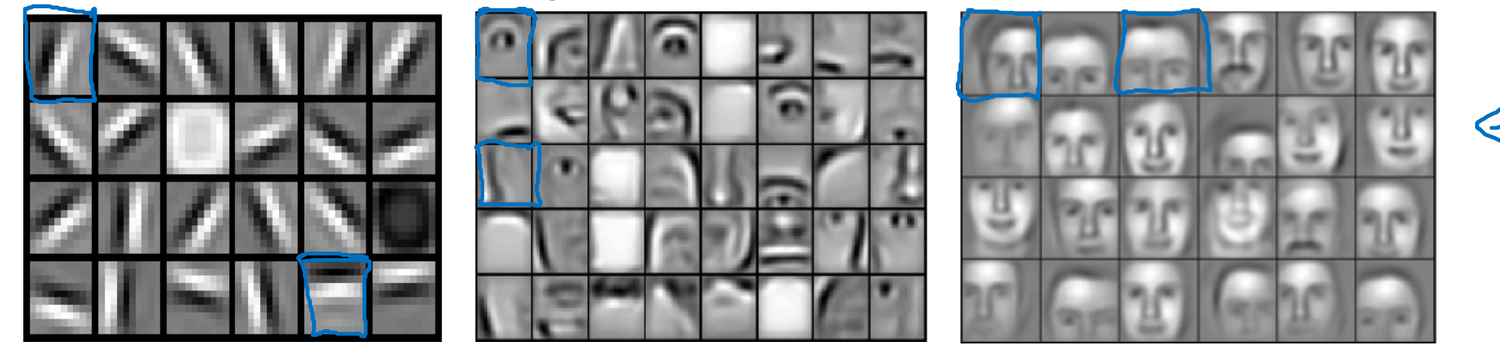
A shallow network can approximate the same function, but it must do in one wide layer what a deep network does in stages — and that turns out to be dramatically more expensive.
Circuit theory: depth saves exponential width
Informally: there are functions a small $L$-layer deep network can compute that a shallow network needs exponentially more hidden units to match. The classic example is the parity function — the XOR of $n$ inputs, $x_1 \oplus x_2 \oplus \cdots \oplus x_n$.
- Deep: build a tree of 2-input XOR units. The tree has depth $O(\log n)$ and only about $n$ units in total.
- Shallow (one hidden layer): with a single hidden layer you must enumerate the input combinations that make the parity odd — on the order of $2^{\,n-1}$ hidden units.
On a log scale the difference is stark: the deep tree's size grows linearly in $n$ while the single hidden layer grows exponentially — a straight line rocketing away.
The exact counts:
| Inputs $n$ | Deep tree — depth $O(\log n)$ | Deep tree — total units $\approx n$ | One hidden layer — units $\approx 2^{\,n-1}$ |
|---|---|---|---|
| $4$ | $2$ | $3$ | $8$ |
| $8$ | $3$ | $7$ | $128$ |
| $16$ | $4$ | $15$ | $32{,}768$ |
| $32$ | $5$ | $31$ | $\approx 2.1 \times 10^{9}$ |
The takeaway. Depth buys expressive efficiency: a few extra layers can replace an exponentially wide single layer. That is a large part of why "deep" networks — rather than merely "wide" ones — became the default. (It is an argument about what is representable cheaply, not a guarantee that training will find it.)
Building blocks: forward and backward functions
To organise the code for an $L$-layer network, think of each layer as two functions that share a small cache. This is the mental model that makes deep backprop tidy.
One layer, two functions
- Forward function (layer $\ell$). Input $a^{[\ell-1]}$; output $a^{[\ell]}$. It computes $z^{[\ell]} = W^{[\ell]}a^{[\ell-1]} + b^{[\ell]}$, $a^{[\ell]} = g^{[\ell]}\left(z^{[\ell]}\right)$, and caches $z^{[\ell]}$ (along with $W^{[\ell]}, b^{[\ell]}$) for the backward pass.
- Backward function (layer $\ell$). Input $da^{[\ell]}$ plus the cached $z^{[\ell]}$; output $da^{[\ell-1]}$ (to hand to the layer before) and the parameter gradients $dW^{[\ell]}, db^{[\ell]}$ (to keep).
Chaining the blocks across the network
Chaining these blocks gives the whole algorithm. Take a concrete three-layer network — ReLU, ReLU, sigmoid — the shape of almost every binary classifier in this reference. The forward pass runs the forward functions $\ell = 1 \dots L$ left to right, each one caching what its partner will need:
The loss then seeds the error, and the backward pass runs the backward functions $\ell = L \dots 1$ — the same chain traversed in reverse, each block consuming its cache, emitting the parameter gradients it owns, and handing $dA^{[\ell-1]}$ to the block before it:
Notice what each half stores. The forward pass caches $z^{[\ell]}$ because the backward function needs the local slope $g^{[\ell]\prime}\left(z^{[\ell]}\right)$ at exactly the point the forward pass passed through; in code it is convenient to cache $W^{[\ell]}, b^{[\ell]}$ alongside it, so a backward block receives everything it needs in one object. And the very last thing the chain produces, $dA^{[0]}$ — how the inputs would like to change — is thrown away: $x$ is data, not a parameter.
Finally every layer takes the gradient-descent step from §6, now once per layer:
Forward and backward propagation for a layer
Here are the two functions written out, for a general layer $\ell$. The forward half is §29; the backward half is Part II's derivation (§25) with the index generalised from ${1,2}$ to any $\ell$.
Forward (layer $\ell$). Input $a^{[\ell-1]}$, output $a^{[\ell]}$, cache $z^{[\ell]}$: $$ z^{[\ell]} = W^{[\ell]} a^{[\ell-1]} + b^{[\ell]}, \qquad a^{[\ell]} = g^{[\ell]}\left(z^{[\ell]}\right). $$
Backward (layer $\ell$). Input $da^{[\ell]}$ and the cached $z^{[\ell]}$; output $da^{[\ell-1]}, dW^{[\ell]}, db^{[\ell]}$:
The last line is what makes it a chain: $da^{[\ell-1]}$ is exactly the input the layer before needs. Substituting it back one step gives the pure recursion in the $dz$'s,
which is the general form of the "push the error back one layer" line first seen at §24.1. Like any recursion it needs a first value, and that value comes from the loss at the output layer — see §33.1 below.
Vectorized over all $m$ examples (uppercase, with the $\tfrac1m$ average and the bias row-sum from §24.2):
dZl  = dAl * gprime_l(Zl)                          # (n_l,   m)   * = element-wise
dWl  = (1/m) * dZl @ A_prev.T                       # (n_l,   n_{l-1})
dbl  = (1/m) * np.sum(dZl, axis=1, keepdims=True)   # (n_l,   1)
dA_prev = Wl.T @ dZl                                # (n_{l-1}, m)   -> input to layer l-1
Every shape is the §30 rule at work: $dW^{[\ell]}$ matches $W^{[\ell]}$ at $(n^{[\ell]}, n^{[\ell-1]})$, $db^{[\ell]}$ matches $b^{[\ell]}$ at $(n^{[\ell]}, 1)$, and $dA^{[\ell-1]}$ comes out $(n^{[\ell-1]}, m)$ — ready for the next backward block.
Seeding the recursion at the output
The backward chain is a recursion, and a recursion needs a first value. That value comes from the loss: differentiate $\mathcal{L}(\hat{y}, y) = -y\log a^{[L]} - (1-y)\log(1 - a^{[L]})$ with respect to the network's own output $a^{[L]} = \hat{y}$.
Feed that $dA^{[L]}$ into the layer-$L$ backward function and the first line does something pleasant. With a sigmoid output, $g^{[L]\prime}\left(z^{[L]}\right) = a^{[L]}(1 - a^{[L]})$, so the messy quotient cancels against the slope and collapses — exactly as proved in §25.1 — to
$$ dZ^{[L]} = dA^{[L]} \odot g^{[L]\prime}\left(Z^{[L]}\right) = A^{[L]} - Y. $$
In practice you skip $dA^{[L]}$ altogether and start the loop at $dZ^{[L]} = A^{[L]} - Y$: one subtraction, no division, and no risk of dividing by an $a^{[L]}$ that has saturated to $0$ or $1$. (Write it out as $dA^{[L]}$ only when the output activation is not sigmoid, since then the cancellation no longer happens.)
With the forward pass of §29, this per-layer backward function is a complete $L$-layer training step: run forward caching each $Z^{[\ell]}$, seed $dZ^{[L]} = A^{[L]} - Y$, run backward for $\ell = L \dots 1$, then update every $W^{[\ell]}, b^{[\ell]}$ with the rule in §32.2.
Parameters versus hyperparameters
Everything trained so far — every $W^{[\ell]}$ and $b^{[\ell]}$ — is a parameter: gradient descent learns it from the data. But look back at the algorithm and you will find a second set of numbers that gradient descent never touches, because you chose them before it ran: the learning rate $\alpha$, how many iterations to run, how many layers $L$, how wide each layer $n^{[\ell]}$ is, which activation $g^{[\ell]}$ to use.
These are the hyperparameters, and the name is precise: they are the knobs that control the parameters. $\alpha$ decides how far each update moves $W^{[\ell]}$; $L$ and $n^{[\ell]}$ decide how many $W^{[\ell]}$'s there are and how big; the choice of $g$ decides the slope $g'$ that the gradient flows through. Change a hyperparameter and you get a different set of learned parameters.
The knobs you set yourself
| Quantity | Symbol | Who sets it | What it controls |
|---|---|---|---|
| Weights | $W^{[1]}, \dots, W^{[L]}$ | learned — gradient descent | the function the network computes |
| Biases | $b^{[1]}, \dots, b^{[L]}$ | learned — gradient descent | each unit's threshold |
| Learning rate | $\alpha$ | you | how far each update step moves |
| Iterations | — | you | how long training runs |
| Number of layers | $L$ | you | the depth of the network |
| Units per layer | $n^{[1]}, \dots, n^{[L-1]}$ | you | the width of each hidden layer |
| Activation choice | $g^{[\ell]}$ | you | the non-linearity, hence $g'$ |
| — and, once the later parts arrive — | |||
| Momentum | $\beta$ | you | how much past gradient carries forward |
| Mini-batch size | — | you | examples per update step |
| Regularization | $\lambda$ | you | how hard overfitting is penalised |
Why the distinction matters. You cannot differentiate the cost with respect to $L$ — "half a layer" is meaningless — so hyperparameters cannot be learned by the same machinery that learns $W$. They have to be searched over: pick values, train, measure, repeat. That outer loop, not the inner gradient-descent loop, is where most of the real work of applied deep learning goes.
Applied deep learning is an empirical process
There is no formula that returns the right $\alpha$ for your problem. What is optimal depends on the data, the architecture, even the hardware — and intuitions transfer poorly across domains, so a learning rate that is excellent for vision may be useless for speech. The honest method is a cycle:
The single most informative experiment is to plot the cost $J$ against the iteration count for a few learning rates. That one picture diagnoses $\alpha$ immediately:
Read the curve, not the theory. If $J$ goes up, $\alpha$ is too large — each step overshoots the minimum and lands further up the far wall of the bowl. If $J$ goes down but barely, $\alpha$ is too small. The useful range is often a factor of ten wide, so search it multiplicatively ($0.001, 0.01, 0.1, \dots$) rather than in equal steps. And re-search it when anything else changes: a network that trained happily at $\alpha = 0.05$ can need a different value after you add a layer, because the same step size now travels through a differently-shaped cost surface.
What does this have to do with the brain?
It is worth collecting the whole algorithm in one place before answering that question, because the answer is essentially "less than the name suggests, and the equations are why."
| Forward propagation | Backward propagation |
|---|---|
| $Z^{[1]} = W^{[1]} X + b^{[1]}$ | $dZ^{[L]} = A^{[L]} - Y$ |
| $A^{[1]} = g^{[1]}\left(Z^{[1]}\right)$ | $dW^{[L]} = \frac{1}{m}\, dZ^{[L]} A^{[L-1]\top}$ |
| $Z^{[2]} = W^{[2]} A^{[1]} + b^{[2]}$ | $db^{[L]} = \frac{1}{m}\, \texttt{np.sum}\left(dZ^{[L]},\ \text{axis}=1,\ \text{keepdims}\right)$ |
| $A^{[2]} = g^{[2]}\left(Z^{[2]}\right)$ | $dZ^{[L-1]} = W^{[L]\top} dZ^{[L]} \odot g^{[L-1]\prime}\left(Z^{[L-1]}\right)$ |
| $\vdots$ | $\vdots$ |
| $A^{[L]} = g^{[L]}\left(Z^{[L]}\right) = \hat{Y}$ | $dZ^{[1]} = W^{[2]\top} dZ^{[2]} \odot g^{[1]\prime}\left(Z^{[1]}\right)$ |
| $dW^{[1]} = \frac{1}{m}\, dZ^{[1]} A^{[0]\top}$ | |
| $db^{[1]} = \frac{1}{m}\, \texttt{np.sum}\left(dZ^{[1]},\ \text{axis}=1,\ \text{keepdims}\right)$ |
A shape check worth doing. The back-propagated error is carried by $W^{[\ell]\top}$, not by $dW^{[\ell]\top}$ — a tempting typo, since the two sit side by side. The shape rule from §30 catches it instantly: both are $(n^{[\ell]}, n^{[\ell-1]})$, so both transpose to a legal shape and NumPy will happily run the wrong one. Reason from meaning instead: $dW$ is a destination (a gradient you keep), $W$ is the road the error travels back along. Likewise $dW^{[1]}$ pairs with $A^{[0]\top} = X^\top$, the activation below layer 1 — never $A^{[1]}$.
The analogy, and where it breaks
Here is the resemblance that gave the field its name. A single unit takes several inputs, combines them, and emits one output if the combination is strong enough — which is roughly what a biological neuron does: dendrites collect signals from other neurons, the cell body integrates them, and if the total crosses a threshold the neuron fires a spike down its axon to the neurons downstream.
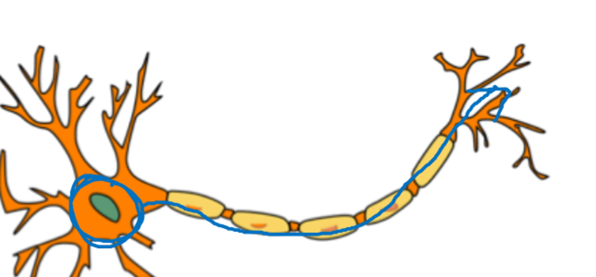
Line the two up and the mapping is easy to state — and easy to over-read:
| Artificial unit | Loose biological counterpart | Where it breaks down |
|---|---|---|
| inputs $x_1, x_2, x_3$ | signals arriving at dendrites | real inputs are spike trains in time, not fixed real numbers |
| weighted sum $w^\top x + b$ | the cell body integrating its inputs | real integration is non-linear, leaky, and stateful |
| activation $g(z)$ | the firing threshold | a neuron emits discrete spikes, not a smooth $g(z)$ |
| output $a$ sent onward | the axon's spike to the next neuron | — |
| learning by backpropagation | ??? | no known biological mechanism |
That last row is the whole story. Forward propagation is a defensible caricature; the learning rule is not. Nobody knows how a real neuron could compute anything like $dW^{[\ell]}$ — backpropagation requires each unit to know the weights of the units above it and to send an error signal precisely backwards along the forward connections, and brains do not appear to do that. Neuroscience has no consensus account of how a single neuron learns, let alone one that matches the equations above.
Why keep the metaphor at all? It is a good first sentence and a bad second one. "It's like a neuron in the brain" gets someone from zero to a mental picture in five seconds, which is why it survives in press releases and introductory lectures. But the deeper you go, the less it earns: the ideas that actually make these networks work — the chain rule, the convexity of the loss, the shapes lining up, the learning rate — come from calculus and optimization, not from biology. This reference is what a neural network is: a composition of matrix multiplies and non-linearities, fitted by gradient descent. The brain inspired it. It does not explain it.
Part IV · The component view
Parts I–III worked with whole vectors and matrices: $z^{[\ell]} = W^{[\ell]}a^{[\ell-1]} + b^{[\ell]}$ hides a great deal of index bookkeeping inside one product. That compression is exactly what makes the equations implementable — but it also means you have never seen which weight multiplies which activation, or why a transpose appears in the backward pass rather than being asserted.
This part drops one level of resolution. Every quantity gets a subscript, every equation is written for a single scalar, and backpropagation is derived from the chain rule one component at a time. Nothing new is proved — every result here collapses back into an equation you already have. What changes is that you can see inside the matrix products, which is the level you need when deriving a new layer type from scratch or when a shape mismatch will not resolve itself.
In one line. A matrix equation is a bundle of scalar equations. Unbundle them, apply the chain rule to each, and re-bundle — the transposes, the outer products, and the $\tfrac{1}{m}$ all appear on their own.
Indices: naming every scalar
A single symbol in a neural network has to answer four questions at once: which layer, which neuron, which training example, and whether the object is a scalar, a vector, or a matrix. The convention already used throughout this reference answers all four, and here we finally use every slot of it.
- Superscript $[\ell]$ — the layer, $\ell = 1, \dots, L$.
- Superscript $(i)$ — the training example, $i = 1, \dots, m$.
- Subscript $j$ or $k$ — the individual neuron. By convention $j$ indexes a neuron of the current layer $\ell$ and $k$ a neuron of the previous layer $\ell-1$.
- Case — a lowercase letter with subscripts is a scalar ($z_j^{[\ell]}$), a lowercase letter without them is a column vector ($z^{[\ell]}$), and a capital is a matrix ($Z^{[\ell]}$, one column per example).
So $a_j^{[\ell]{}(i)}$ is one number: the activation of neuron $j$ in layer $\ell$ for example $i$. Its column is $a^{[\ell]{}(i)}$, and stacking those columns for all $m$ examples gives $A^{[\ell]}$.
One symbol needs care. Up to now $L$ has meant the number of layers, and it also commonly denotes the loss. From here on the loss on one example is $\mathcal{L}$ and the cost over the batch is $J = \tfrac{1}{m}\sum_i \mathcal{L}^{(i)}$, exactly as in §5 — never $L$, which remains the depth.
| Concept | One component | Vector / matrix | Meaning |
|---|---|---|---|
| Indices and sizes | |||
| Layer index | $[\ell]$ | — | $\ell = 1, \dots, L$; layer $0$ is the input |
| Example index | $(i)$ | — | $i = 1, \dots, m$ |
| Neuron index | $j$, $k$ | — | $j$ in layer $\ell$; $k$ in layer $\ell-1$ |
| Layer width | $n^{[\ell]}$ | — | units in layer $\ell$; $n^{[0]} = n_x$ |
| Forward — activations | |||
| Input | $x_k^{(i)} = a_k^{[0]{}(i)}$ | $x^{(i)} \in \mathbb{R}^{n^{[0]}}$, $X = A^{[0]} \in \mathbb{R}^{n^{[0]} \times m}$ | feature $k$ of example $i$ |
| Pre-activation | $z_j^{[\ell]{}(i)}$ | $z^{[\ell]{}(i)} \in \mathbb{R}^{n^{[\ell]}}$, $Z^{[\ell]} \in \mathbb{R}^{n^{[\ell]} \times m}$ | weighted sum plus bias, before $g$ |
| Activation | $a_j^{[\ell]{}(i)}$ | $a^{[\ell]{}(i)} \in \mathbb{R}^{n^{[\ell]}}$, $A^{[\ell]} \in \mathbb{R}^{n^{[\ell]} \times m}$ | output of neuron $j$, after $g$ |
| Forward — parameters (no $(i)$: shared across examples) | |||
| Weight | $w_{j,k}^{[\ell]}$ | $W^{[\ell]} \in \mathbb{R}^{n^{[\ell]} \times n^{[\ell-1]}}$ | from neuron $k$ of layer $\ell-1$ into neuron $j$ of layer $\ell$ |
| Weight row | — | $w_j^{[\ell]} \in \mathbb{R}^{1 \times n^{[\ell-1]}}$ | row $j$ of $W^{[\ell]}$: every weight feeding neuron $j$ |
| Bias | $b_j^{[\ell]}$ | $b^{[\ell]} \in \mathbb{R}^{n^{[\ell]}}$ | one offset per neuron |
| Activation function | $g^{[\ell]}(\cdot)$ | — | applied element-wise; may differ per layer |
| Backward — gradients ($d\,\square$ means $\partial \mathcal{L} / \partial \square$) | |||
| Activation gradient | $da_j^{[\ell]{}(i)}$ | $da^{[\ell]{}(i)} \in \mathbb{R}^{n^{[\ell]}}$, $dA^{[\ell]} \in \mathbb{R}^{n^{[\ell]} \times m}$ | the signal arriving from layer $\ell+1$ |
| Pre-activation gradient | $dz_j^{[\ell]{}(i)}$ | $dz^{[\ell]{}(i)} \in \mathbb{R}^{n^{[\ell]}}$, $dZ^{[\ell]} \in \mathbb{R}^{n^{[\ell]} \times m}$ | the shared error signal at neuron $j$ |
| Weight gradient | $\dfrac{\partial \mathcal{L}}{\partial w_{j,k}^{[\ell]}}$ | $dW^{[\ell]} \in \mathbb{R}^{n^{[\ell]} \times n^{[\ell-1]}}$ | same shape as $W^{[\ell]}$ |
| Bias gradient | $\dfrac{\partial \mathcal{L}}{\partial b_j^{[\ell]}}$ | $db^{[\ell]} \in \mathbb{R}^{n^{[\ell]}}$ | same shape as $b^{[\ell]}$ |
| Loss, cost, and operators | |||
| Loss (one example) | $\mathcal{L}^{(i)}$ | — | error on example $i$ alone |
| Cost (the batch) | $J$ | — | $J = \frac{1}{m}\sum_{i=1}^{m} \mathcal{L}^{(i)}$ — the source of every $\frac{1}{m}$ |
| Hadamard product | $\odot$ | — | element-wise multiplication |
| Ones vector | — | $\mathbf{1}_m \in \mathbb{R}^{m}$ | sums across the example columns |
The distinction between the loss $\mathcal{L}^{(i)}$ and the cost $J$ is worth pausing on, because it is the entire origin of the $\tfrac{1}{m}$ factors in §33. Each example produces its own loss and therefore its own gradient for every parameter. The cost averages those losses, so the parameter gradient is the average of the per-example gradients. Activation gradients carry no $\tfrac{1}{m}$: each example keeps its own error signal all the way back.
Here is the whole apparatus on a concrete network — three inputs, two hidden layers of four units, and two outputs — drawn for one example $i$, so every activation carries $(i)$ while no weight or bias does.
Inside one neuron
The circles above hide the two operations every neuron performs. Unfold one — neuron $3$ of hidden layer $1$ — and the forward pass becomes elementary arithmetic: scale each incoming activation by its weight, add them together with the bias, then apply $g$.
Written out, that neuron computes a dot product followed by a shift:
Notice which indices the sum runs over. The neuron $j$ is fixed; the sum sweeps $k$ across every neuron of the previous layer. That is the row of $W^{[\ell]}$ belonging to neuron $j$, dotted with the incoming activation column — which is precisely why the matrix form is a product.
The matrices, entry by entry
Now stack those scalars. The layout convention is fixed once and never varies: for parameters, row = destination, column = source; for anything indexed by examples, rows are neurons, columns are examples.
Every example-indexed object shares one layout. The input matrix, the pre-activations, and the activations are all "neurons down, examples across":
Bias broadcasting, written honestly
In $Z^{[\ell]} = W^{[\ell]}A^{[\ell-1]} + b^{[\ell]}$ the product already has shape $(n^{[\ell]}, m)$, but $b^{[\ell]}$ is only $(n^{[\ell]}, 1)$. NumPy's broadcasting (§15) silently copies the bias across all $m$ columns. The exact statement of what it copies is an outer product with a row of ones:
So the fully explicit forward pass is $Z^{[\ell]} = W^{[\ell]}A^{[\ell-1]} +
b^{[\ell]}\mathbf{1}_m^\top$, and in code it stays one line, Z = W @ A_prev + b. Keep the
$\mathbf{1}_m$ in mind — it returns in §39.2, where the same
ones vector is what sums the bias gradient back down to one column.
Backpropagation, component by component
Now the derivation. Backpropagation was stated at the matrix level in §33 and motivated by a two-layer computation graph in §25; here it is obtained from the chain rule applied to individual scalars, which is where the transposes come from.
Before the algebra, the picture. The forward pass sends information left to right; the backward pass sends an error signal right to left, along the very same edges, scaled by the very same weights.
The four scalar derivatives
Assume the signal $da_j^{[\ell]} = \partial\mathcal{L}/\partial a_j^{[\ell]}$ has already arrived from the layer above (the example index $(i)$ is suppressed — every line below is for one example). Four derivatives follow, each a direct application of the chain rule.
One. The activation acts on each neuron independently: $a_j^{[\ell]} = g^{[\ell]}(z_j^{[\ell]})$ involves no other neuron. So the chain rule contributes exactly one local factor, the slope of $g$ at that neuron's own pre-activation:
Because each $j$ is scaled by its own slope and nothing else, collecting these over $j$ gives an element-wise product, not a matrix one. That is the origin of the $\odot$.
Two. The weight $w_{j,k}^{[\ell]}$ appears in the pre-activation of §37 exactly once — inside $z_j^{[\ell]}$, multiplying $a_k^{[\ell-1]}$. So $\partial z_j^{[\ell]} / \partial w_{j,k}^{[\ell]} = a_k^{[\ell-1]}$ and
In words: a weight's gradient is the error at the neuron it feeds, times the activation it carried. A weight that pushed a large input into a badly wrong neuron gets a large gradient — exactly the parameter most worth changing.
Three. The bias enters $z_j^{[\ell]}$ additively, so $\partial z_j^{[\ell]} / \partial b_j^{[\ell]} = 1$ and the factor simply vanishes:
Four. The last one is different, and it is the only place addition appears.
Why one gradient is a sum
An activation $a_k^{[\ell-1]}$ does not feed one neuron of the next layer — it feeds every one of them. The loss therefore depends on it through $n^{[\ell]}$ separate paths, and the multivariable chain rule says: add up what comes back along each path.
Since $\partial z_j^{[\ell]} / \partial a_k^{[\ell-1]} = w_{j,k}^{[\ell]}$, summing the paths gives
That last observation is the transpose. In the forward pass, computing $z_j$ meant summing over $k$ — along a row of $W^{[\ell]}$. In the backward pass, computing $da_k$ means summing over $j$ — down a column. Same numbers, other index summed, hence $W^{[\ell]\top}$. The transpose is not a trick to make the shapes fit; it is the statement that a weight carries signal forward and error backward through the same connection.
One neuron's backward pass
All four results, on the neuron we opened up earlier. One incoming gradient enters, one shared error signal is formed, and everything else is that signal multiplied by a local factor.
Note the economy that makes backpropagation cheap: $dz_j^{[\ell]}$ is computed once and reused by all three downstream quantities. A naive implementation would re-multiply the whole chain from the loss down to each individual weight; backpropagation multiplies it once per layer and shares the result.
From components back to matrices
Re-bundle the four scalar results and the matrix equations of §33 appear — now derived rather than asserted.
Collecting the indices
| Step | Component form | Collected form (one example) | Why that operation |
|---|---|---|---|
| through the activation | $dz_j^{[\ell]} = da_j^{[\ell]}\, g^{[\ell]\prime}(z_j^{[\ell]})$ | $dz^{[\ell]} = da^{[\ell]} \odot g^{[\ell]\prime}(z^{[\ell]})$ | each $j$ uses its own slope — element-wise |
| weight gradient | $\dfrac{\partial \mathcal{L}}{\partial w_{j,k}^{[\ell]}} = dz_j^{[\ell]} a_k^{[\ell-1]}$ | $dW^{[\ell]} = dz^{[\ell]} \left(a^{[\ell-1]}\right)^{\top}$ | one free index $j$, one free index $k$ — an outer product |
| bias gradient | $\dfrac{\partial \mathcal{L}}{\partial b_j^{[\ell]}} = dz_j^{[\ell]}$ | $db^{[\ell]} = dz^{[\ell]}$ | the local derivative is $1$ |
| pass back | $da_k^{[\ell-1]} = \sum_j dz_j^{[\ell]} w_{j,k}^{[\ell]}$ | $da^{[\ell-1]} = \left(W^{[\ell]}\right)^{\top} dz^{[\ell]}$ | the sum runs over $j$, not $k$ — a transpose |
The shapes confirm each line. The outer product is $(n^{[\ell]}, 1) \times (1, n^{[\ell-1]}) = (n^{[\ell]}, n^{[\ell-1]})$, matching $W^{[\ell]}$ as any weight gradient must. The pass-back is $(n^{[\ell-1]}, n^{[\ell]}) \times (n^{[\ell]}, 1) = (n^{[\ell-1]}, 1)$ — a column for the previous layer, exactly the input its own §38.1 expects. This is the §30 habit at work, one index at a time.
Where the $\tfrac{1}{m}$ and the ones vector come from
Everything so far concerned one example. The batch is trained on the cost $J = \tfrac{1}{m}\sum_i \mathcal{L}^{(i)}$, so each parameter gradient is the average of its per-example gradients:
Both sums over $i$ are performed for free by matrix algebra. In $dZ^{[\ell]} \left(A^{[\ell-1]}\right)^{\top}$ the inner dimension is $m$, so forming the product contracts the example index away — the summation over examples is the matrix multiplication. For the bias there is no second matrix to contract against, so the sum is written with the ones vector from §37.2, now used in the opposite direction: $\mathbf{1}_m^\top$ copied the bias out across columns; $\mathbf{1}_m$ sums the gradient back in.
In NumPy the ones vector is spelled np.sum(..., axis=1, keepdims=True), which is the same
contraction: db = (1/m) * np.sum(dZ, axis=1, keepdims=True).
The whole sweep, in code
Chain the layer functions and the algorithm is complete: a forward pass that caches, a backward sweep that consumes the caches from last layer to first, and one update.
# forward: cache what the backward pass will need
caches = {}
A = X                                            # A[0] = X
for l in range(1, L + 1):
    A_prev = A
    Z = W[l] @ A_prev + b[l]                     # broadcast bias  (comp-eq-broadcast)
    A = g[l](Z)
    caches[l] = (A_prev, W[l], Z)                # a^(l-1), W^(l), z^(l)

# backward: seed at the output, then sweep down
grads = {}
dA = A - Y                                       # dZ^[L] seed for sigmoid + cross-entropy
for l in reversed(range(1, L + 1)):
    A_prev, Wl, Z = caches[l]
    dZ = dA * g_prime[l](Z)                       # element-wise   (the odot)
    grads[f"dW{l}"] = (1 / m) * dZ @ A_prev.T     # outer product, examples contracted
    grads[f"db{l}"] = (1 / m) * dZ.sum(axis=1, keepdims=True)
    dA = Wl.T @ dZ                                # the transpose  -> input to layer l-1

# update every parameter
for l in range(1, L + 1):
    W[l] -= alpha * grads[f"dW{l}"]
    b[l] -= alpha * grads[f"db{l}"]
One caveat in that seed. The line
dA = A - Yis really $dZ^{[L]}$, not $dA^{[L]}$ — it is the collapsed form that only holds for a sigmoid output with the cross-entropy loss (§33.1). Writing it intodAand then multiplying byg_prime[L](Z)on the first iteration would apply the sigmoid slope twice. Real implementations either seeddZdirectly and skip the first activation step, or seed the honest $dA^{[L]}$ of §40. The shortcut above is the common one and the common bug.
The output seed, for any number of outputs
Every backward step assumes $da^{[\ell]}$ is already known. The recursion's first value comes from differentiating the loss with respect to the network's own output.
For binary classification the output layer has $n^{[L]} = 1$ neuron, $a_1^{[L]{}(i)} = \hat{y}^{(i)}$ is a predicted probability, and the loss is the cross-entropy of §5.1. Differentiating it with respect to that one activation gives the seed already met in §33.1.
For several outputs — multi-label prediction, or one unit per class — nothing changes except that each output neuron carries its own seed, indexed by $j$:
Stack those scalars in the standard layout — neurons down, examples across — and the seed for the whole batch is one element-wise expression on two $(n^{[L]}, m)$ matrices:
When $n^{[L]} = 1$ both matrices collapse to a single row of $m$ predictions and $m$ labels, and — because the output is a sigmoid — the whole expression collapses one step further, to $dZ^{[L]} = A^{[L]} - Y$. That is the complete cycle: predict forward, measure the loss, seed the gradient at the output, and propagate it back to every parameter.
Where this goes next
The pieces above are a complete, trainable $L$-layer classifier: a forward pass (§29), shapes that catch most bugs before they run (§30), a reason to prefer depth (§31), the building-block/cache view (§32), the general per-layer backward function (§33), and the knobs you tune around it (§34) — with Part IV supplying the component-level derivation underneath all of it. Each block is reusable, so extending this reference is a matter of appending new parts that lean on the same notation and the same forward/backward machinery. Natural next topics:
- Regularization — $L_2$ / dropout, to stop the network memorising the training set.
- Optimization — mini-batches, momentum, RMSProp, Adam; better than plain gradient descent on real data.
- Tuning & normalization — learning-rate schedules, batch norm, and how to set the hyperparameters.
House style for new parts. Keep one
##per topic with an explicit{#id}; wrap every display equation, figure, and table in a:::captionblock; draw computation graphs withneuralflow(forward left-to-right, backward as a red mirror); and write math as KaTeX, words in prose. Numbering and the§N.Mcross-references continue automatically across parts.